Tag Archives: mathematics

Amplitudes 2023 Retrospective

I’m back from CERN this week, with a bit more time to write, so I thought I’d share some thoughts about last week’s Amplitudes conference.

One thing I got wrong in last week’s post: I’ve now been told only 213 people actually showed up in person, as opposed to the 250-ish estimate I had last week. This may seem fewer than Amplitudes in Prague had, but it seems likely they had a few fewer show up than appeared on the website. Overall, the field is at least holding steady from year to year, and definitely has grown since the pandemic (when 2019’s 175 was already a very big attendance).

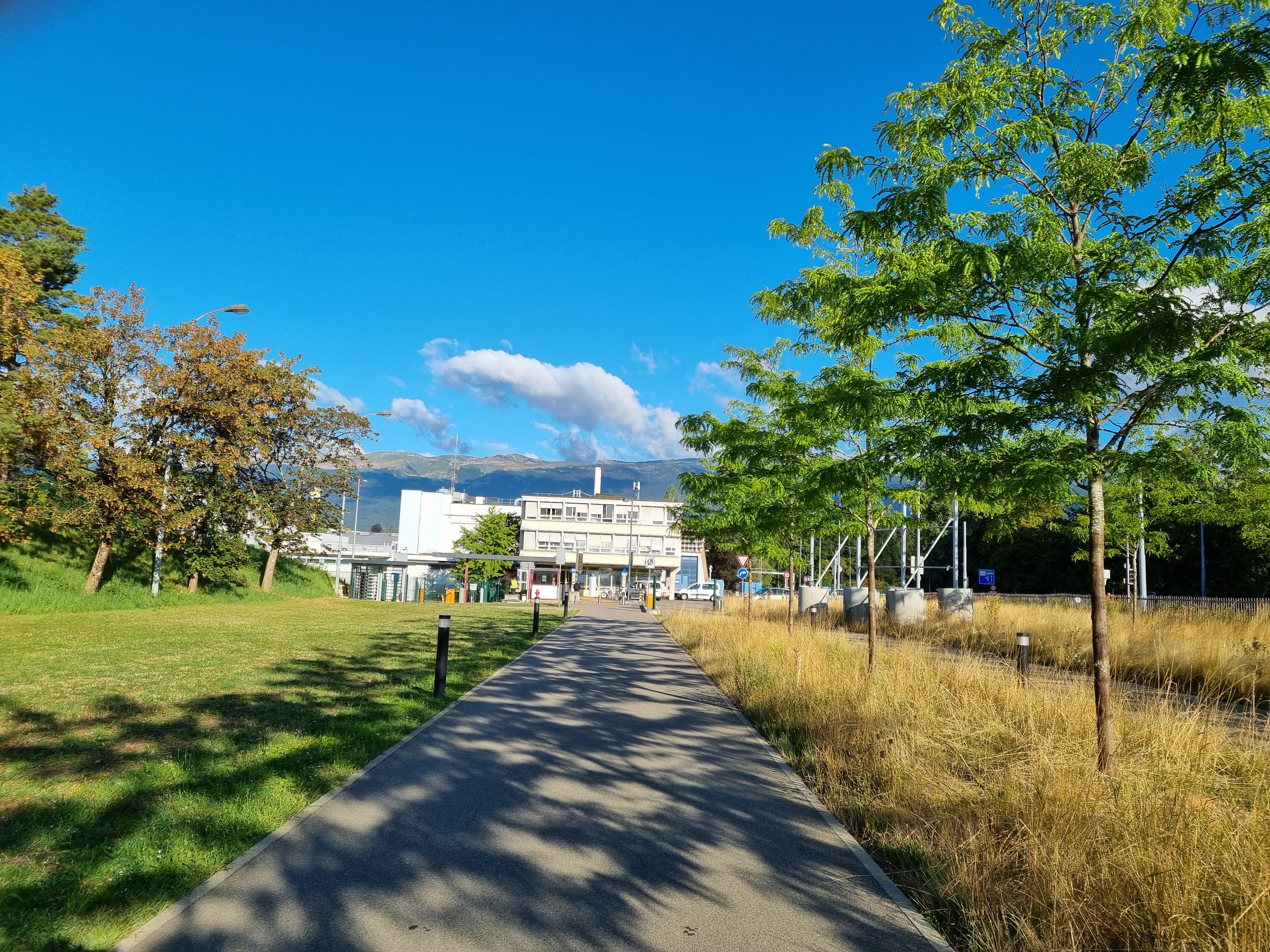
It was cool having a conference in CERN proper, surrounded by the history of European particle physics. The lecture hall had an abstract particle collision carved into the wood, and the visitor center would in principle have had Standard Model coffee mugs were they not sold out until next May. (There was still enough other particle physics swag, Swiss chocolate, and Swiss chocolate that was also particle physics swag.) I’d planned to stay on-site at the CERN hostel, but I ended up appreciated not doing that: the folks who did seemed to end up a bit cooped up by the end of the conference, even with the conference dinner as a chance to get out.

Past Amplitudes conferences have had associated public lectures. This time we had a not-supposed-to-be-public lecture, a discussion between Nima Arkani-Hamed and Beate Heinemann about the future of particle physics. Nima, prominent as an amplitudeologist, also has a long track record of reasoning about what might lie beyond the Standard Model. Beate Heinemann is an experimentalist, one who has risen through the ranks of a variety of different particle physics experiments, ending up well-positioned to take a broad view of all of them.

It would have been fun if the discussion erupted into an argument, but despite some attempts at provocative questions from the audience that was not going to happen, as Beate and Nima have been friends for a long time. Instead, they exchanged perspectives: on what’s coming up experimentally, and what theories could explain it. Both argued that it was best to have many different directions, a variety of experiments covering a variety of approaches. (There wasn’t any evangelism for particular experiments, besides a joking sotto voce mention of a muon collider.) Nima in particular advocated that, whether theorist or experimentalist, you have to have some belief that what you’re doing could lead to a huge breakthrough. If you think of yourself as just a “foot soldier”, covering one set of checks among many, then you’ll lose motivation. I think Nima would agree that this optimism is irrational, but necessary, sort of like how one hears (maybe inaccurately) that most new businesses fail, but someone still needs to start businesses.

Michelangelo Mangano’s talk on Thursday covered similar ground, but with different emphasis. He agrees that there are still things out there worth discovering: that our current model of the Higgs, for instance, is in some ways just a guess: a simplest-possible answer that doesn’t explain as much as we’d like. But he also emphasized that Standard Model physics can be “new physics” too. Just because we know the model doesn’t mean we can calculate its consequences, and there are a wealth of results from the LHC that improve our models of protons, nuclei, and the types of physical situations they partake in, without changing the Standard Model.

We saw an impressive example of this in Gregory Korchemsky’s talk on Wednesday. He presented an experimental mystery, an odd behavior in the correlation of energies of jets of particles at the LHC. These jets can include a very large number of particles, enough to make it very hard to understand them from first principles. Instead, Korchemsky tried out our field’s favorite toy model, where such calculations are easier. By modeling the situation in the limit of a very large number of particles, he was able to reproduce the behavior of the experiment. The result was a reminder of what particle physics was like before the Standard Model, and what it might become again: partial models to explain odd observations, a quest to use the tools of physics to understand things we can’t just a priori compute.

On the other hand, amplitudes does do a priori computations pretty well as well. Fabrizio Caola’s talk opened the conference by reminding us just how much our precise calculations can do. He pointed out that the LHC has only gathered 5% of its planned data, and already it is able to rule out certain types of new physics to fairly high energies (by ruling out indirect effects, that would show up in high-precision calculations). One of those precise calculations featured in the next talk, by Guilio Gambuti. (A FORM user, his diagrams were the basis for the header image of my Quanta article last winter.) Tiziano Peraro followed up with a technique meant to speed up these kinds of calculations, a trick to simplify one of the more computationally intensive steps in intersection theory.

The rest of Monday was more mathematical, with talks by Zeno Capatti, Jaroslav Trnka, Chia-Kai Kuo, Anastasia Volovich, Francis Brown, Michael Borinsky, and Anna-Laura Sattelberger. Borinksy’s talk felt the most practical, a refinement of his numerical methods complete with some actual claims about computational efficiency. Francis Brown discussed an impressively powerful result, a set of formulas that manages to unite a variety of invariants of Feynman diagrams under a shared explanation.

Tuesday began with what I might call “visitors”: people from adjacent fields with an interest in amplitudes. Alday described how the duality between string theory in AdS space and super Yang-Mills on the boundary can be used to get quite concrete information about string theory, calculating how the theory’s amplitudes are corrected by the curvature of AdS space using a kind of “bootstrap” method that felt nicely familiar. Tim Cohen talked about a kind of geometric picture of theories that extend the Standard Model, including an interesting discussion of whether it’s really “geometric”. Marko Simonovic explained how the integration techniques we develop in scattering amplitudes can also be relevant in cosmology, especially for the next generation of “sky mappers” like the Euclid telescope. This talk was especially interesting to me since this sort of cosmology has a significant presence at CEA Paris-Saclay. Along those lines an interesting paper, “Cosmology meets cohomology”, showed up during the conference. I haven’t had a chance to read it yet!

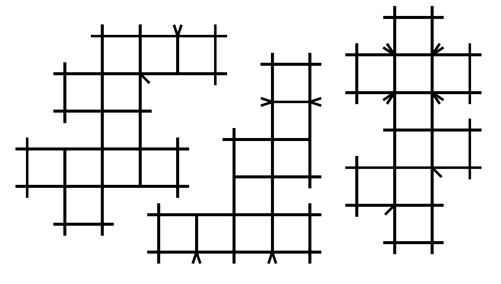
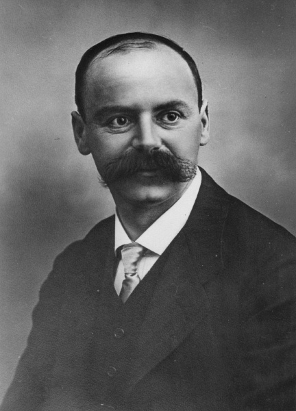
Just before lunch, we had David Broadhurst give one of his inimitable talks, complete with number theory, extremely precise numerics, and literary and historical references (apparently, Källén died flying his own plane). He also remedied a gap in our whimsically biological diagram naming conventions, renaming the pedestrian “double-box” as a (in this context, Orwellian) lobster. Karol Kampf described unusual structures in a particular Effective Field Theory, while Henriette Elvang’s talk addressed what would become a meaningful subtheme of the conference, where methods from the mathematical field of optimization help amplitudes researchers constrain the space of possible theories. Giulia Isabella covered another topic on this theme later in the day, though one of her group’s selling points is managing to avoid quite so heavy-duty computations.

The other three talks on Tuesday dealt with amplitudes techniques for gravitational wave calculations, as did the first talk on Wednesday. Several of the calculations only dealt with scattering black holes, instead of colliding ones. While some of the results can be used indirectly to understand the colliding case too, a method to directly calculate behavior of colliding black holes came up again and again as an important missing piece.

The talks on Wednesday had to start late, owing to a rather bizarre power outage (the lights in the room worked fine, but not the projector). Since Wednesday was the free afternoon (home of quickly sold-out CERN tours), this meant there were only three talks: Veneziano’s talk on gravitational scattering, Korchemsky’s talk, and Nima’s talk. Nima famously never finishes on time, and this time attempted to control his timing via the surprising method of presenting, rather than one topic, five “abstracts” on recent work that he had not yet published. Even more surprisingly, this almost worked, and he didn’t run too ridiculously over time, while still managing to hint at a variety of ways that the combinatorial lessons behind the amplituhedron are gradually yielding useful perspectives on more general realistic theories.

Thursday, Andrea Puhm began with a survey of celestial amplitudes, a topic that tries to build the same sort of powerful duality used in AdS/CFT but for flat space instead. They’re gradually tackling the weird, sort-of-theory they find on the boundary of flat space. The two next talks, by Lorenz Eberhardt and Hofie Hannesdottir, shared a collaborator in common, namely Sebastian Mizera. They also shared a common theme, taking a problem most people would have assumed was solved and showing that approaching it carefully reveals extensive structure and new insights.

Cristian Vergu, in turn, delved deep into the literature to build up a novel and unusual integration method. We’ve chatted quite a bit about it at the Niels Bohr Institute, so it was nice to see it get some attention on the big stage. We then had an afternoon of trips beyond polylogarithms, with talks by Anne Spiering, Christoph Nega, and Martijn Hidding, each pushing the boundaries of what we can do with our hardest-to-understand integrals. Einan Gardi and Ruth Britto finished the day, with a deeper understanding of the behavior of high-energy particles and a new more mathematically compatible way of thinking about “cut” diagrams, respectively.

On Friday, João Penedones gave us an update on a technique with some links to the effective field theory-optimization ideas that came up earlier, one that “bootstraps” whole non-perturbative amplitudes. Shota Komatsu talked about an intriguing variant of the “planar” limit, one involving large numbers of particles and a slick re-writing of infinite sums of Feynman diagrams. Grant Remmen and Cliff Cheung gave a two-parter on a bewildering variety of things that are both surprisingly like, and surprisingly unlike, string theory: important progress towards answering the question “is string theory unique?”

Friday afternoon brought the last three talks of the conference. James Drummond had more progress trying to understand the symbol letters of supersymmetric Yang-Mills, while Callum Jones showed how Feynman diagrams can apply to yet another unfamiliar field, the study of vortices and their dynamics. Lance Dixon closed the conference without any Greta Thunberg references, but with a result that explains last year’s mystery of antipodal duality. The explanation involves an even more mysterious property called antipodal self-duality, so we’re not out of work yet!

At Amplitudes 2023 at CERN

I’m at the big yearly conference of my sub-field this week, called Amplitudes. This year, surprisingly for the first time, it’s at the very appropriate location of CERN.

Somewhat overshadowed by the very picturesque Alps

Amplitudes keeps on growing. In 2019, we had 175 participants. We were on Zoom in 2020 and 2021, with many more participants, but that probably shouldn’t count. In Prague last year we had 222. This year, I’ve been told we have even more, something like 250 participants (the list online is bigger, but includes people joining on Zoom). We’ve grown due to new students, but also new collaborations: people from adjacent fields who find the work interesting enough to join along. This year we have mathematicians talking about D-modules, bootstrappers finding new ways to get at amplitudes in string theory, beyond-the-standard-model theorists talking about effective field theories, and cosmologists talking about the large-scale structure of the universe.

The talks have been great, from clear discussions of earlier results to fresh-off-the-presses developments, plenty of work in progress, and even one talk where the speaker’s opinion changed during the coffee break. As we’re at CERN, there’s also a through-line about the future of particle physics, with a chat between Nima Arkani-Hamed and the experimentalist Beate Heinemann on Tuesday and a talk by Michelangelo Mangano about the meaning of “new physics” on Thursday.

I haven’t had a ton of time to write, I keep getting distracted by good discussions! As such, I’ll do my usual thing, and say a bit more about specific talks in next week’s post.

Cabinet of Curiosities: The Deluxe Train Set

I’ve got a new paper out this week with Andrew McLeod. I’m thinking of it as another entry in this year’s “cabinet of curiosities”, interesting Feynman diagrams with unusual properties. Although this one might be hard to fit into a cabinet.

Over the past few years, I’ve been finding Feynman diagrams with interesting connections to Calabi-Yau manifolds, the spaces originally studied by string theorists to roll up their extra dimensions. With Andrew and other collaborators, I found an interesting family of these diagrams called traintracks, which involve higher-and-higher dimensional manifolds as they get longer and longer.

This time, we started hooking up our traintracks together.

We call diagrams like these traintrack network diagrams, or traintrack networks for short. The original traintracks just went “one way”: one family, going higher in Calabi-Yau dimension the longer they got. These networks branch out, one traintrack leading to another and another.

In principle, these are much more complicated diagrams. But we find we can work with them in almost the same way. We can find the same “starting point” we had for the original traintracks, the set of integrals used to find the Calabi-Yau manifold. We’ve even got more reliable tricks, a method recently honed by some friends of ours that consistently find a Calabi-Yau manifold inside the original traintracks.

Surprisingly, though, this isn’t enough.

It works for one type of traintrack network, a so-called “cross diagram” like this:

But for other diagrams, if the network branches any more, the trick stops working. We still get an answer, but that answer is some more general space, not just a Calabi-Yau manifold.

That doesn’t mean that these general traintrack networks don’t involve Calabi-Yaus at all, mind you: it just means this method doesn’t tell us one way or the other. It’s also possible that simpler versions of these diagrams, involving fewer particles, will once again involve Calabi-Yaus. This is the case for some similar diagrams in two dimensions. But it’s starting to raise a question: how special are the Calabi-Yau related diagrams? How general do we expect them to be?

Another fun thing we noticed has to do with differential equations. There are equations that relate one diagram to another simpler one. We’ve used them in the past to build up “ladders” of diagrams, relating each picture to one with one of its boxes “deleted”. We noticed, playing with these traintrack networks, that these equations do a bit more than we thought. “Deleting” a box can make a traintrack short, but it can also chop a traintrack in half, leaving two “dangling” pieces, one on either side.

This reminded me of an important point, one we occasionally lose track of. The best-studied diagrams related to Calabi-Yaus are called “sunrise” diagrams. If you squish together a loop in one of those diagrams, the whole diagram squishes together, becoming much simpler. Because of that, we’re used to thinking of these as diagrams with a single “geometry”, one that shows up when you don’t “squish” anything.

Traintracks, and traintrack networks, are different. “Squishing” the diagram, or “deleting” a box, gives you a simpler diagram, but not much simpler. In particular, the new diagram will still contain traintracks, and traintrack networks. That means that we really should think of each traintrack network not just as one “top geometry”, but of a collection of geometries, different Calabi-Yaus that break into different combinations of Calabi-Yaus in different ways. It’s something we probably should have anticipated, but the form these networks take is a good reminder, one that points out that we still have a lot to do if we want to understand these diagrams.

Solutions and Solutions

The best misunderstandings are detective stories. You can notice when someone is confused, but digging up why can take some work. If you manage, though, you learn much more than just how to correct the misunderstanding. You learn something about the words you use, and the assumptions you make when using them.

Recently, someone was telling me about a book they’d read on Karl Schwarzschild. Schwarzschild is famous for discovering the equations that describe black holes, based on Einstein’s theory of gravitation. To make the story more dramatic, he did so only shortly before dying from a disease he caught fighting in the first World War. But this person had the impression that Schwarzschild had done even more. According to this person, the book said that Schwarzschild had done something to prove Einstein’s theory, or to complete it.

Another Schwarzschild accomplishment: that mustache

At first, I thought the book this person had read was wrong. But after some investigation, I figured out what happened.

The book said that Schwarzschild had found the first exact solution to Einstein’s equations. That’s true, and as a physicist I know precisely what it means. But I now realize that the average person does not.

In school, the first equations you solve are algebraic, x+y=z. Some equations, like x^2=4, have solutions. Others, like x^2=-4, seem not to, until you learn about new types of numbers that solve them. Either way, you get used to equations being like a kind of puzzle, a question for which you need to find an answer.

If you’re thinking of equations like that, then it probably sounds like Schwarzschild “solved the puzzle”. If Schwarzschild found the first solution to Einstein’s equation, that means that Einstein did not. That makes it sound like Einstein’s work was incomplete, that he had asked the right question but didn’t yet know the right answer.

Einstein’s equations aren’t algebraic equations, though. They’re differential equations. Instead of equations for a variable, they’re equations for a mathematical function, a formula that, in this case, describes the curvature of space and time.

Scientists in many fields use differential equations, but they use them in different ways. If you’re a chemist or a biologist, it might be that you’re most used to differential equations with simple solutions, like sines, cosines, or exponentials. You learn how to solve these equations, and they feel a bit like the algebraic ones: you have a puzzle, and then you solve the puzzle.

Other fields, though, have tougher differential equations. If you’re a physicist or an engineer, you’ve likely met differential equations that you can’t treat in this way. If you’re dealing with fluid mechanics, or general relativity, or even just Newtonian gravity in an odd situation, you can’t usually solve the problem by writing down known functions like sines and cosines.

That doesn’t mean you can’t solve the problem at all, though!

Even if you can’t write down a solution to a differential equation with sines and cosines, a solution can still exist. (In some cases, we can even prove a solution exists!) It just won’t be written in terms of sines and cosines, or other functions you’ve learned in school. Instead, the solution will involve some strange functions, functions no-one has heard of before.

If you want, you can make up names for those functions. But unless you’re going to classify them in a useful way, there’s not much point. Instead, you work with these functions by approximation. You calculate them in a way that doesn’t give you the full answer, but that does let you estimate how close you are. That’s good enough to give you numbers, which in turn is good enough to compare to experiments. With just an approximate solution, like this, Einstein could check if his equations described the orbit of Mercury.

Once you know you can find these approximate solutions, you have a different perspective on equations. An equation isn’t just a mysterious puzzle. If you can approximate the solution, then you already know how to solve that puzzle. So we wouldn’t think of Einstein’s theory as incomplete because he was only able to find approximate solutions: for a theory as complicated as Einstein’s, that’s perfectly normal. Most of the time, that’s all we need.

But it’s still pretty cool when you don’t have to do this. Sometimes, we can not just approximate, but actually “write down” the solution, either using known functions or well-classified new ones. We call a solution like that an analytic solution, or an exact solution.

That’s what Schwarzschild managed. These kinds of exact solutions often only work in special situations, and Schwarzschild’s is no exception. His Schwarzschild solution works for matter in a special situation, arranged in a perfect sphere. If matter happened to be arranged in that way, then the shape of space and time would be exactly as Schwarzschild described it.

That’s actually pretty cool! Einstein’s equations are complicated enough that no-one was sure that there were any solutions like that, even in very special situations. Einstein expected it would be a long time until they could do anything except approximate solutions.

(If Schwarzschild’s solution only describes matter arranged in a perfect sphere, why do we think it describes real black holes? This took later work, by people like Roger Penrose, who figured out that matter compressed far enough will always find a solution like Schwarzschild’s.)

Schwarzschild intended to describe stars with his solution, or at least a kind of imaginary perfect star. What he found was indeed a good approximation to real stars, but also the possibility that a star shoved into a sufficiently small space would become something weird and new, something we would come to describe as a black hole. That’s a pretty impressive accomplishment, especially for someone on the front lines of World War One. And if you know the difference between an exact solution and an approximate one, you have some idea of what kind of accomplishment that is.

What’s a Cosmic String?

Nowadays, we have telescopes that detect not just light, but gravitational waves. We’ve already learned quite a bit about astrophysics from these telescopes. They observe ripples coming from colliding black holes, giving us a better idea of what kinds of black holes exist in the universe. But the coolest thing a gravitational wave telescope could discover is something that hasn’t been seen yet: a cosmic string.

This art is from an article in Symmetry magazine which is, as far as I can tell, not actually about cosmic strings.

You might have heard of cosmic strings, but unless you’re a physicist you probably don’t know much about them. They’re a prediction, coming from cosmology, of giant string-like objects floating out in space.

That might sound like it has something to do with string theory, but it doesn’t actually have to, you can have these things without any string theory at all. Instead, you might have heard that cosmic strings are some kind of “cracks” or “wrinkles” in space-time. Some articles describe this as like what happens when ice freezes, cracks forming as water settles into a crystal.

That description, in terms of ice forming cracks between crystals, is great…if you’re a physicist who already knows how ice forms cracks between crystals. If you’re not, I’m guessing reading those kinds of explanations isn’t helpful. I’m guessing you’re still wondering why there ought to be any giant strings floating in space.

The real explanation has to do with a type of mathematical gadget physicists use, called a scalar field. You can think of a scalar field as described by a number, like a temperature, that can vary in space and time. The field carries potential energy, and that energy depends on what the scalar field’s “number” is. Left alone, the field settles into a situation with as little potential energy as it can, like a ball rolling down a hill. That situation is one of the field’s default values, something we call a “vacuum” value. Changing the field away from its vacuum value can take a lot of energy. The Higgs boson is one example of a scalar field. Its vacuum value is the value it has in day to day life. In order to make a detectable Higgs boson at the Large Hadron Collider, they needed to change the field away from its vacuum value, and that took a lot of energy.

In the very early universe, almost back at the Big Bang, the world was famously in a hot dense state. That hot dense state meant that there was a lot of energy to go around, so scalar fields could vary far from their vacuum values, pretty much randomly. As the universe expanded and cooled, there was less and less energy available for these fields, and they started to settle down.

Now, the thing about these default, “vacuum” values of a scalar field is that there doesn’t have to be just one of them. Depending on what kind of mathematical function the field’s potential energy is, there could be several different possibilities each with equal energy.

Let’s imagine a simple example, of a field with two vacuum values: +1 and -1. As the universe cooled down, some parts of the universe would end up with that scalar field number equal to +1, and some to -1. But what happens in between?

The scalar field can’t just jump from -1 to +1, that’s not allowed in physics. It has to pass through 0 in between. But, unlike -1 and +1, 0 is not a vacuum value. When the scalar field number is equal to 0, the field has more energy than it does when it’s equal to -1 or +1. Usually, a lot more energy.

That means the region of scalar field number 0 can’t spread very far: the further it spreads, the more energy it takes to keep it that way. On the other hand, the region can’t vanish altogether: something needs to happen to transition between the numbers -1 and +1.

The thing that happens is called a domain wall. A domain wall is a thin sheet, as thin as it can physically be, where the scalar field doesn’t take its vacuum value. You can roughly think of it as made up of the scalar field, a churning zone of the kind of bosons the LHC was trying to detect.

This sheet still has a lot of energy, bound up in the unusual value of the scalar field, like an LHC collision in every proton-sized chunk. As such, like any object with a lot of energy, it has a gravitational field. For a domain wall, the effect of this gravity would be very very dramatic: so dramatic, that we’re pretty sure they’re incredibly rare. If they were at all common, we would have seen evidence of them long before now!

Ok, I’ve shown you a wall, that’s weird, sure. What does that have to do with cosmic strings?

The number representing a scalar field doesn’t have to be a real number: it can be imaginary instead, or even complex. Now I’d like you to imagine a field with vacuum values on the unit circle, in the complex plane. That means that +1 and -1 are still vacuum values, but so are e^{i \pi/2}, and e^{3 i \pi/2}, and everything else you can write as e^{i\theta}. However, 0 is still not a vacuum value. Neither is, for example, 2 e^{i\pi/3}.

With vacuum values like this, you can’t form domain walls. You can make a path between -1 and +1 that only goes through the unit circle, through e^{i \pi/2} for example. The field will be at its vacuum value throughout, taking no extra energy.

However, imagine the different regions form a circle. In the picture above, suppose that the blue area at the bottom is at vacuum value -1 and red is at +1. You might have e^{i \pi/2} in the green region, and e^{3 i \pi/2} in the purple region, covering the whole circle smoothly as you go around.

Now, think about what happens in the middle of the circle. On one side of the circle, you have -1. On the other, +1. (Or, on one side e^{i \pi/2}, on the other, e^{3 i \pi/2}). No matter what, different sides of the circle are not allowed to be next to each other, you can’t just jump between them. So in the very middle of the circle, something else has to happen.

Once again, that something else is a field that goes away from its vacuum value, that passes through 0. Once again, that takes a lot of energy, so it occupies as little space as possible. But now, that space isn’t a giant wall. Instead, it’s a squiggly line: a cosmic string.

Cosmic strings don’t have as dramatic a gravitational effect as domain walls. That means they might not be super-rare. There might be some we haven’t seen yet. And if we do see them, it could be because they wiggle space and time, making gravitational waves.

Cosmic strings don’t require string theory, they come from a much more basic gadget, scalar fields. We know there is one quite important scalar field, the Higgs field. The Higgs vacuum values aren’t like +1 and -1, or like the unit circle, though, so the Higgs by itself won’t make domain walls or cosmic strings. But there are a lot of proposals for scalar fields, things we haven’t discovered but that physicists think might answer lingering questions in particle physics, and some of those could have the right kind of vacuum values to give us cosmic strings. Thus, if we manage to detect cosmic strings, we could learn something about one of those lingering questions.

AI Is the Wrong Sci-Fi Metaphor

Over the last year, some people felt like they were living in a science fiction novel. Last November, the research laboratory OpenAI released ChatGPT, a program that can answer questions on a wide variety of topics. Last month, they announced GPT-4, a more powerful version of ChatGPT’s underlying program. Already in February, Microsoft used GPT-4 to add a chatbot feature to its search engine Bing, which journalists quickly managed to use to spin tales of murder and mayhem.

For those who have been following these developments, things don’t feel quite so sudden. Already in 2019, AI Dungeon showed off how an early version of GPT could be used to mimic an old-school text-adventure game, and a tumblr blogger built a bot that imitates his posts as a fun side project. Still, the newer programs have shown some impressive capabilities.

Are we close to “real AI”, to artificial minds like the positronic brains in Isaac Asimov’s I, Robot? I can’t say, in part because I’m not sure what “real AI” really means. But if you want to understand where things like ChatGPT come from, how they work and why they can do what they do, then all the talk of AI won’t be helpful. Instead, you need to think of an entirely different set of Asimov novels: the Foundation series.

While Asimov’s more famous I, Robot focused on the science of artificial minds, the Foundation series is based on a different fictional science, the science of psychohistory. In the stories, psychohistory is a kind of futuristic social science. In the real world, historians and sociologists can find general principles of how people act, but don’t yet have the kind of predictive theories physicists or chemists do. Foundation imagines a future where powerful statistical methods have allowed psychohistorians to precisely predict human behavior: not yet that of individual people, but at least the average behavior of civilizations. They can not only guess when an empire is soon to fall, but calculate how long it will be before another empire rises, something few responsible social scientists would pretend to do today.

GPT and similar programs aren’t built to predict the course of history, but they do predict something: given part of a text, they try to predict the rest. They’re called Large Language Models, or LLMs for short. They’re “models” in the sense of mathematical models, formulas that let us use data to make predictions about the world, and the part of the world they model is our use of language.

Normally, a mathematical model is designed based on how we think the real world works. A mathematical model of a pandemic, for example, might use a list of people, each one labeled as infected or not. It could include an unknown number, called a parameter, for the chance that one person infects another. That parameter would then be filled in, or fixed, based on observations of the pandemic in the real world.

LLMs (as well as most of the rest of what people call “AI” these days) are a bit different. Their models aren’t based on what we expect about the real world. Instead, they’re in some sense “generic”, models that could in principle describe just about anything. In order to make this work, they have a lot more parameters, tons and tons of flexible numbers that can get fixed in different ways based on data.

(If that part makes you a bit uncomfortable, it bothers me too, though I’ve mostly made my peace with it.)

The surprising thing is that this works, and works surprisingly well. Just as psychohistory from the Foundation novels can predict events with much more detail than today’s historians and sociologists, LLMs can predict what a text will look like much more precisely than today’s literature professors. That isn’t necessarily because LLMs are “intelligent”, or because they’re “copying” things people have written. It’s because they’re mathematical models, built by statistically analyzing a giant pile of texts.

Just as Asimov’s psychohistory can’t predict the behavior of individual people, LLMs can’t predict the behavior of individual texts. If you start writing something, you shouldn’t expect an LLM to predict exactly how you would finish. Instead, LLMs predict what, on average, the rest of the text would look like. They give a plausible answer, one of many, for what might come next.

They can’t do that perfectly, but doing it imperfectly is enough to do quite a lot. It’s why they can be used to make chatbots, by predicting how someone might plausibly respond in a conversation. It’s why they can write fiction, or ads, or college essays, by predicting a plausible response to a book jacket or ad copy or essay prompt.

LLMs like GPT were invented by computer scientists, not social scientists or literature professors. Because of that, they get described as part of progress towards artificial intelligence, not as progress in social science. But if you want to understand what ChatGPT is right now, and how it works, then that perspective won’t be helpful. You need to put down your copy of I, Robot and pick up Foundation. You’ll still be impressed, but you’ll have a clearer idea of what could come next.

Building the Railroad to Rigor

As a kid who watched far too much educational television, I dimly remember learning about the USA’s first transcontinental railroad. Somehow, parts of the story stuck with me. Two companies built the railroad from different directions, one from California and the other from the middle of the country, aiming for a mountain in between. Despite the US Civil War happening around this time, the two companies built through, in the end racing to where the final tracks were laid with a golden spike.

I’m a theoretical physicist, so of course I don’t build railroads. Instead, I build new mathematical methods, ways to check our theories of particle physics faster and more efficiently. Still, something of that picture resonates with me.

You might think someone who develops new mathematical methods would be a mathematician, not a physicist. But while there are mathematicians who work on the problems I work on, their goals are a bit different. They care about rigor, about stating only things they can carefully prove. As such, they often need to work with simplified examples, “toy models” well-suited to the kinds of theorems they can build.

Physicists can be a bit messier. We don’t always insist on the same rigor the mathematicians do. This makes our results less reliable, but it makes our “toy models” a fair amount less “toy”. Our goal is to try to tackle questions closer to the actual real world.

What happens when physicists and mathematicians work on the same problem?

If the physicists worked alone, they might build and build, and end up with an answer that isn’t actually true. The mathematicians, keeping rigor in mind, would be safe in the truth of what they built, but might not end up anywhere near the physicists’ real-world goals.

Together, though, physicists and mathematicians can build towards each other. The physicists can keep their eyes on the mathematicians, correcting when they notice something might go wrong and building more and more rigor into their approach. The mathematicians can keep their eyes on the physicists, building more and more complex applications of their rigorous approaches to get closer and closer to the real world. Eventually, like the transcontinental railroad, the two groups meet: the mathematicians prove a rigorous version of the physicists’ approach, or the physicists adopt the mathematicians’ ideas and apply them to their own theories.

A sort of conference photo

In practice, it isn’t just two teams, physicists and mathematicians, building towards each other. Different physicists themselves work with different levels of rigor, aiming to understand different problems in different theories, and the mathematicians do the same. Each of us is building our own track, watching the other tracks build towards us on the horizon. Eventually, we’ll meet, and science will chug along over what we’ve built.

At Geometries and Special Functions for Physics and Mathematics in Bonn

I’m at a workshop this week. It’s part of a series of “Bethe Forums”, cozy little conferences run by the Bethe Center for Theoretical Physics in Bonn.

You can tell it’s an institute for theoretical physics because they have one of these, but not a “doing room”

The workshop’s title, “Geometries and Special Functions for Physics and Mathematics”, covers a wide range of topics. There are talks on Calabi-Yau manifolds, elliptic (and hyper-elliptic) polylogarithms, and cluster algebras and cluster polylogarithms. Some of the talks are by mathematicians, others by physicists.

In addition to the talks, this conference added a fun innovative element, “my favorite problem sessions”. The idea is that a speaker spends fifteen minutes introducing their “favorite problem”, then the audience spends fifteen minutes discussing it. Some treated these sessions roughly like short talks describing their work, with the open directions at the end framed as their favorite problem. Others aimed broader, trying to describe a general problem and motivate interest in people of other sub-fields.

This was a particularly fun conference for me, because the seemingly distinct topics all connect in one way or another to my own favorite problem. In our “favorite theory” of N=4 super Yang-Mills, we can describe our calculations in terms of an “alphabet” of pieces that let us figure out predictions almost “by guesswork”. These alphabets, at least in the cases we know how to handle, turn out to correspond to mathematical structures called cluster algebras. If we look at interactions of six or seven particles, these cluster algebras are a powerful guide. For eight or nine, they still seem to matter, but are much harder to use.

For ten particles, though, things get stranger. That’s because ten particles is precisely where elliptic curves, and their related elliptic polylogarithms, show up. Things then get yet more strange, and with twelve particles or more we start seeing Calabi-Yau manifolds magically show up in our calculations.

We don’t know what an “alphabet” should look like for these Calabi-Yau manifolds (but I’m working on it). Because of that, we don’t know how these cluster algebras should appear.

In my view, any explanation for the role of cluster algebras in our calculations has to extend to these cases, to elliptic polylogarithms and Calabi-Yau manifolds. Without knowing how to frame an alphabet for these things, we won’t be able to solve the lingering mysteries that fill our field.

Because of that, “my favorite problem” is one of my biggest motivations, the question that drives a large chunk of what I do. It’s what’s made this conference so much fun, and so stimulating: almost every talk had something I wanted to learn.

Cabinet of Curiosities: The Train-Ladder

I’ve got a new paper out this week, with Andrew McLeod, Roger Morales, Matthias Wilhelm, and Chi Zhang. It’s yet another entry in this year’s “cabinet of curiosities”, quirky Feynman diagrams with interesting traits.

A while back, I talked about a set of Feynman diagrams I could compute with any number of “loops”, bypassing the approximations we usually need to use in particle physics. That wasn’t the first time someone did that. Back in the 90’s, some folks figured out how to do this for so-called “ladder” diagrams. These diagrams have two legs on one end for two particles coming in, two legs on the other end for two particles going out, and a ladder in between, like so:

There are infinitely many of these diagrams, but they’re all beautifully simple, variations on a theme that can be written down in a precise mathematical way.

Change things a little bit, though, and the situation gets wildly more intractable. Let the rungs of the ladder peek through the sides, and you get something looking more like the tracks for a train:

These traintrack integrals are much more complicated. Describing them requires the mathematics of Calabi-Yau manifolds, involving higher and higher dimensions as the tracks get longer. I don’t think there’s any hope of understanding these things for all loops, at least not any time soon.

What if we aimed somewhere in between? A ladder that just started to turn traintrack?

Add just a single pair of rungs, and it turns out that things remain relatively simple. If we do this, it turns out we don’t need any complicated Calabi-Yau manifolds. We just need the simplest Calabi-Yau manifold, called an elliptic curve. It’s actually the same curve for every version of the diagram. And the situation is simple enough that, with some extra cleverness, it looks like we’ve found a trick to calculate these diagrams to any number of loops we’d like.

(Another group figured out the curve, but not the calculation trick. They’ve solved different problems, though, studying all sorts of different traintrack diagrams. They sorted out some confusion I used to have about one of those diagrams, showing it actually behaves precisely the way we expected it to. All in all, it’s been a fun example of the way different scientists sometimes hone in on the same discovery.)

These developments are exciting, because Feynman diagrams with elliptic curves are still tough to deal with. We still have whole conferences about them. These new elliptic diagrams can be a long list of test cases, things we can experiment with with any number of loops. With time, we might truly understand them as well as the ladder diagrams!

This Week at Quanta Magazine

I’ve got an article in Quanta Magazine this week, about a program called FORM.

Quanta has come up a number of times on this blog, they’re a science news outlet set up by the Simons Foundation. Their goal is to enhance the public understanding of science and mathematics. They cover topics other outlets might find too challenging, and they cover the topics others cover with more depth. Most people I know who’ve worked with them have been impressed by their thoroughness: they take fact-checking to a level I haven’t seen with other science journalists. If you’re doing a certain kind of mathematical work, then you hope that Quanta decides to cover it.

A while back, as I was chatting with one of their journalists, I had a startling realization: if I want Quanta to cover something, I can send them a tip, and if they’re interested they’ll write about it. That realization resulted in the article I talked about here. Chatting with the journalist interviewing me for that article, though, I learned something if anything even more startling: if I want Quanta to cover something, and I want to write about it, I can pitch the article to Quanta, and if they’re interested they’ll pay me to write about it.

Around the same time, I happened to talk to a few people in my field, who had a problem they thought Quanta should cover. A software, called FORM, was used in all the most serious collider physics calculations. Despite that, the software wasn’t being supported: its future was unclear. You can read the article to learn more.

One thing I didn’t mention in that article: I hadn’t used FORM before I started writing it. I don’t do those “most serious collider physics calculations”, so I’d never bothered to learn FORM. I mostly use Mathematica, a common choice among physicists who want something easy to learn, even if it’s not the strongest option for many things.

(By the way, it was surprisingly hard to find quotes about FORM that didn’t compare it specifically to Mathematica. In the end I think I included one, but believe me, there could have been a lot more.)

Now, I wonder if I should have been using FORM all along. Many times I’ve pushed to the limits of what Mathematica could comfortable handle, the limits of what my computer’s memory could hold, equations long enough that just expanding them out took complicated work-arounds. If I had learned FORM, maybe I would have breezed through those calculations, and pushed even further.

I’d love it if this article gets FORM more attention, and more support. But also, I’d love it if it gives a window on the nuts and bolts of hard-core particle physics: the things people have to do to turn those T-shirt equations into predictions for actual colliders. It’s a world in between physics and computer science and mathematics, a big part of the infrastructure of how we know what we know that, precisely because it’s infrastructure, often ends up falling through the cracks.

Edit: For researchers interested in learning more about FORM, the workshop I mentioned at the end of the article is now online, with registrations open.