Tag Archives: quantum field theory

How (Not) to Sum the Natural Numbers: Zeta Function Regularization

$1+2+3+4+5+6+\ldots=-\frac{1}{12}$

If you follow Numberphile on YouTube or Bad Astronomy on Slate you’ve already seen this counter-intuitive sum written out. Similarly, if you follow those people or Sciencetopia’s Good Math, Bad Math, you’re aware that the way that sum was presented by Numberphile in that video was seriously flawed.

There is a real sense in which adding up all of the natural numbers (numbers 1, 2, 3…) really does give you minus twelve, despite all the reasons this should be impossible. However, there is also a real sense in which it does not, and cannot, do any such thing. To explain this, I’m going to introduce two concepts: complex analysis and regularization.

This discussion is not going to be mathematically rigorous, but it should give an authentic and accurate view of where these results come from. If you’re interested in the full mathematical details, a later discussion by Numberphile should help, and the mathematically confident should read Terence Tao’s treatment from back in 2010.

With that said, let’s talk about sums! Well, one sum in particular:

$\frac{1}{1^s}+\frac{1}{2^s}+\frac{1}{3^s}+\frac{1}{4^s}+\frac{1}{5^s}+\frac{1}{6^s}+\ldots = \zeta(s)$

If s is greater than one, then each term in this infinite sum gets smaller and smaller fast enough that you can add them all up and get a number. That number is referred to as $\zeta(s)$ , the Riemann Zeta Function.

So what if s is smaller than one?

The infinite sum that I described doesn’t converge for s less than one. Add it up in any reasonable way, and it just approaches infinity. Put another way, the sum is not properly defined. But despite this, $\zeta(s)$ is not infinite for s less than one!

Now as you might object, we only defined the Riemann Zeta Function for s greater than one. How do we know anything at all about it for s less than one?

That is where complex analysis comes in. Complex analysis sounds like a made-up term for something unreasonably complicated, but it’s quite a bit more approachable when you know what it means. Analysis is the type of mathematics that deals with functions, infinite series, and the basis of calculus. It’s often contrasted with Algebra, which usually considers mathematical concepts that are discrete rather than smooth (this definition is a huge simplification, but it’s not very relevant to this post). Complex means that complex analysis deals with functions, not of everyday real numbers, but of complex numbers, or numbers with an imaginary part.

So what does complex analysis say about the Riemann Zeta Function?

One of the most impressive results of complex analysis is the discovery that if a function of a complex number is sufficiently smooth (the technical term is analytic) then it is very highly constrained. In particular, if you know how the function behaves over an area (technical term: open set), then you know how it behaves everywhere else!

If you’re expecting me to explain why this is true, you’ll be disappointed. This is serious mathematics, and serious mathematics isn’t the sort of thing you can give the derivation for in a few lines. It takes as much effort and knowledge to replicate a mathematical result as it does to replicate many lab results in science.

What I can tell you is that this sort of approach crops up in many places, and is part of a general theme. There is a lot you can tell about a mathematical function just by looking at its behavior in some limited area, because mathematics is often much more constrained than it appears. It’s the same sort of principle behind the work I’ve been doing recently.

In the case of the Riemann Zeta Function, we have a definition for s greater than one. As it turns out, this definition still works if s is a complex number, as long as the real part of s is greater than one. Using this information, the value of the Riemann Zeta Function for a large area (half of the complex numbers), complex analysis tells us its value for every other number. In particular, it tells us this:

$\zeta(-1)= -\frac{1}{12}$

If the Riemann Zeta Function is consistently defined for every complex number, then it must have this value when s is minus one.

If we still trusted the sum definition for this value of s, we could plug in -1 and get

$1+2+3+4+5+6+\ldots=-\frac{1}{12}$

Does that make this statement true? Sort of. It all boils down to a concept from physics called regularization.

In physics, we know that in general there is no such thing as infinity. With a few exceptions, nothing in nature should be infinite, and finite evidence (without mathematical trickery) should never lead us to an infinite conclusion.

Despite this, occasionally calculations in physics will give infinite results. Almost always, this is evidence that we are doing something wrong: we are not thinking hard enough about what’s really going on, or there is something we don’t know or aren’t taking into account.

Doing physics research isn’t like taking a physics class: sometimes, nobody knows how to do the problem correctly! In many cases where we find infinities, we don’t know enough about “what’s really going on” to correct them. That’s where regularization comes in handy.

Regularization is the process by which an infinite result is replaced with a finite result (made “regular”), in a way so that it keeps the same properties. These finite results can then be used to do calculations and make predictions, and so long as the final predictions are regularization independent (that is, the same if you had done a different regularization trick instead) then they are legitimate.

In string theory, one way to compute the required dimensions of space and time ends up giving you an infinite sum, a sum that goes 1+2+3+4+5+…. In context, this result is obviously wrong, so we regularize it. In particular, we say that what we’re really calculating is the Riemann Zeta Function, which we happen to be evaluating at -1. Then we replace 1+2+3+4+5+… with -1/12.

Now remember when I said that getting infinities is a sign that you’re doing something wrong? These days, we have a more rigorous way to do this same calculation in string theory, one that never forces us to take an infinite sum. As expected, it gives the same result as the old method, showing that the old calculation was indeed regularization independent.

Sometimes we don’t have a better way of doing the calculation, and that’s when regularization techniques come in most handy. A particular family of tricks called renormalization is quite important, and I’ll almost certainly discuss it in a future post.

So can you really add up all the natural numbers and get -1/12? No. But if a calculation tells you to add up all the natural numbers, and it’s obvious that the result can’t be infinite, then it may secretly be asking you to calculate the Riemann Zeta Function at -1. And that, as we know from complex analysis, is indeed -1/12.

Update on the Amplituhedron

2 Replies

Awhile back I wrote a post on the Amplituhedron, a type of mathematical object found by Nima Arkani-Hamed and Jaroslav Trnka that can be used to do calculations of scattering amplitudes in planar N=4 super Yang-Mills theory. (Scattering amplitudes are formulas used to calculate probabilities in particle physics, from the probability that an unstable particle will decay to the probability that a new particle could be produced by a collider.) Since then, they published two papers on the topic, the most recent of which came out the day before New Year’s Eve. These papers laid out the amplituhedron concept in some detail, and answered a few lingering questions. The latest paper focused on one particular formula, the probability that two particles bounce off each other. In discussing this case, the paper serves two purposes:

1. Demonstrating that Arkani-Hamed and Trnka did their homework.

2. Showing some advantages of the amplituhedron setup.

Let’s talk about them one at a time.

Doing their homework

There’s already a lot known about N=4 super Yang-Mills theory. In order to propose a new framework like the amplituhedron, Arkani-Hamed and Trnka need to show that the new framework can reproduce the old knowledge. Most of the paper is dedicated to doing just that. In several sections Arkani-Hamed and Trnka show that the amplituhedron reproduces known properties of the amplitude, like the behavior of its logarithm, its collinear limit (the situation when two momenta in the calculation become parallel), and, of course, unitarity.

What, you heard the amplituhedron “removes” unitarity? How did unitarity get back in here?

This is something that has confused several commenters, both here and on Ars Technica, so it bears some explanation.

Unitarity is the principle that enforces the laws of probability. In its simplest form, unitarity requires that all probabilities for all possible events add up to one. If this seems like a pretty basic and essential principle, it is! However, it and locality (the idea that there is no true “action at a distance”, that particles must meet to interact) can be problematic, causing paradoxes for some approaches to quantum gravity. Paradoxes like these inspired Arkani-Hamed to look for ways to calculate scattering amplitudes that don’t rely on locality and unitarity, and with the amplituhedron he succeeded.

However, just because the amplituhedron doesn’t rely on unitarity and locality, doesn’t mean it violates them. The amplituhedron, for all its novelty, still calculates quantities in N=4 super Yang-Mills. N=4 super Yang-Mills is well understood, it’s well-behaved and cuddly, and it obeys locality and unitarity.

This is why the amplituhedron is not nearly as exciting as a non-physicist might think. The amplituhedron, unlike most older methods, isn’t based on unitarity and locality. However, the final product still has to obey unitarity and locality, because it’s the same final product that others calculate through other means. So it’s not as if we’ve completely given up on basic principles of physics.

Not relying on unitarity and locality is valuable. For those who research scattering amplitudes, it has often been useful to try to “eliminate” one principle or another from our calculations. 20 years ago, avoiding Feynman diagrams was the key to finding dramatic simplifications. Now, many different approaches try to sidestep different principles. (For example, while the amplituhedron calculates an integrand and leaves a final integral to be done, I’m working on approaches that never employ an integrand.)

If we can avoid relying on some “basic” principle, that’s usually good evidence that the principle might be a consequence of something even more basic. By showing how unitarity can arise from the amplituhedron, Arkani-Hamed and Trnka have shown that a seemingly basic principle can come out of a theory that doesn’t impose it.

Advantages of the Amplituhedron

Not all of the paper compares to old results and principles, though. A few sections instead investigate novel territory, and in doing so show some of the advantages and disadvantages of the amplituhedron.

Last time I wrote on this topic, I was unclear on whether the amplituhedron was more efficient than existing methods. At this point, it appears that it is not. While the formula that the amplituhedron computes has been found by other methods up to seven loops, the amplituhedron itself can only get up to three loops or so in practical cases. (Loops are a way that calculations are classified in particle physics. More loops means a more complex calculation, and a more precise final result.)

The amplituhedron’s primary advantage is not in efficiency, but rather in the fact that its mathematical setup makes it straightforward to derive interesting properties for any number of loops desired. As Trnka occasionally puts it, the central accomplishment of the amplituhedron is to find “the question to which the amplitude is the answer”. By being able to phrase this “question” mathematically, one can be very general, which allows them to discover several properties that should hold no matter how complex the rest of the calculation becomes. It also has another implication: if this mathematical question has a complete mathematical answer, that answer could calculate the amplitude for any number of loops. So while the amplituhedron is not more efficient than other methods now, it has the potential to be dramatically more efficient if it can be fully understood.

All that said, it’s important to remember that the amplituhedron is still limited in scope. Currently, it applies to a particular theory, one that doesn’t (and isn’t meant to) describe the real world. It’s still too early to tell whether similar concepts can be defined for more realistic theories. If they can, though, it won’t depend on supersymmetry or string theory. One of the most powerful techniques for making predictions for the Large Hadron Collider, the technique of generalized unitarity, was first applied to N=4 super Yang-Mills. While the amplituhedron is limited now, I would not be surprised if it (and its competitors) give rise to practical techniques ten or twenty years down the line. It’s happened before, after all.

The Parke-Taylor Amplitudes: Why Quantum Field Theory Might Not Be So Hard, After All

2 Replies

If you’ve been following my blog for a while, you know that Quantum Field Theory is hard work. To calculate anything, you have to draw an ever-increasing number of diagrams, translate them into formulas involving the momentum and energy of your particles, and add all those formulas up to get your final result, the amplitude of the process you’re interested in.

As I said in that post, my area of research involves trying to find patterns in the results of these calculations, patterns that make doing the calculation simpler. With that in mind, you might wonder why we expect to find any patterns in the first place. If Quantum Field Theory is so complicated, what insurance do we have that it can be made simpler? Where does the motivation come from?

Our motivation comes from a series of discoveries that show that things really do simplify, often in unexpected ways. I won’t go through all of these discoveries here, but I want to tell you about one of the first discoveries that showed amplitudes researchers that they were on the right track.

Let’s try to calculate a comparatively simple process. Say that we’ve got two gluons (force carrying bosons for the strong force, an example of a Yang-Mills field). Suppose the two gluons collide, and some number of gluons emerge. It could be two again, or it could be three, or more.

For now, let’s just think about diagrams at tree level, that is, diagrams with no loops. The particles can travel from place to place in the diagram, but they can’t form closed loops on the inside.

Gluons have two types of interactions, places where particle lines can come together. You can either have three lines meeting at one point, or four.

If two gluons come in and two come out, we have four possible diagrams:

4ptMHV

Note that while the last diagram looks like it has a loop in it (in the form of the triangle in the middle), actually that triangle just represents that two particles are passing each other without colliding, so that their lines cross.

The number of diagrams increases substantially as you increase the number of outgoing particles. With two particles going to three particles, you get fifteen diagrams. Here are three examples:

5ptMHV

Since the number of diagrams just keeps increasing, you’d expect the final amplitude to become more and more complicated as well. However, Steven Parke and Tomasz Taylor found in 1986 that for a particular arrangement of the spins of the particles (for technical people: this is the Maximally Helicity Violating configuration, or two particles with negative helicity and all the rest with positive helicity) the answer simplifies dramatically. In the sort of variables we use these days, the result can be expressed in an incredibly simple form:

$\frac{\langle 1 | 2 \rangle^4}{ \langle 1 | 2 \rangle\langle 2 | 3 \rangle\langle 3 | 4 \rangle \ldots \langle n-1 | n \rangle\langle n | 1 \rangle}$

Here the angle brackets represent momenta of the incoming (for 1 and 2) and outgoing (all the other numbers) particles, with n being the total number of particles (two going in, and however many going out). (Technically, these are spinor-helicity variables, and those interested in the technical details should check out chapter 3 of this or chapter 2 of this.)

Nowadays, we know why this amplitude looks so simple, in terms of something called B C F W recursion. At the time though, it was quite extraordinary.

This is the sort of simplification we keep running into when studying amplitudes. Almost always, it means that there is some deeper principle that we don’t yet understand, something that would let us do our calculations much faster and more efficiently. It indicates that Quantum Field Theory might not be so hard after all.

What are Vacua? (A Point about the String Landscape)

4 Replies

A couple weeks back, there was a bit of a scuffle between Matt Strassler and Peter Woit on the subject of predictions in string theory (or more properly, the question of whether any predictions can be made at all). As a result, Strassler has begun a series on the subject of quantum field theory, string theory, and predictions.

Strassler hasn’t gotten to the topic of string vacua yet, but he’s probably going to cover the subject in a future post. While his take on the subject is likely to be more expansive and precise than mine, I think my perspective on the problem might still be of interest.

Let’s start with the basics: one of the problems often cited with string theory is the landscape problem, the idea that string theory has a metaphorical landscape of around 10^500 vacua.

What are vacua?

Vacua is the plural of vacuum.

Ok, and?

A vacuum is empty space.

That’s what you thought, right? That’s the normal meaning of vacuum. But if a vacuum is empty, how can there be more than one of them, let alone 10^500?

“Empty” is subjective.

Now we’re getting somewhere. The problem with defining a concept like “empty space” in string theory or field theory is that it’s unclear what precisely it should be empty of. Naively, such a space should be empty of “stuff”, or “matter”, but our naive notions of “matter” don’t apply to field theory or string theory. In fact, there is plenty of “stuff” that can be present in “empty” space.

Think about two pieces of construction paper. One is white, the other is yellow. Which is empty? Neither has anything drawn on it, so while one has a color and the other does not, both are empty.

“Empty space” doesn’t come in multiple colors like construction paper, but there are equivalent parameters that can vary. In quantum field theory, one option is for scalar fields to take different values. In string theory, different dimensions can be curled up in different ways (as an aside, when string theory leads to a quantum field theory often these different curling-up shapes correspond to different values for scalar fields, so the two ideas are related).

So if space can have “stuff” in it and still count as empty, are there any limits on what can be in it?

As it turns out, there is a quite straightforward limit. But to explain it, I need to talk a bit about why physicists care about vacua in the first place.

Why do physicists care about vacua?

In physics, there is a standard modus operandi for solving problems. If you’ve taken even a high school physics course, you’ve probably encountered it in some form. It’s not the only way to solve problems, but it’s one of the easiest. The idea, broadly, is the following:

First get the initial conditions, and then use the laws of physics to see what happens next.

In high school physics, this is how almost every problem works: your teacher tells you what the situation is, and you use what you know to figure out what happens next.

In quantum field theory, things are a bit more subtle, but there is a strong resemblance. You start with a default state, and then find the perturbations, or small changes, around that state.

In high school, your teacher told you what the initial conditions were. In quantum field theory, you need another source for the “default state”. Sometimes, you get that from observations of the real world. Sometimes, though, you want to make a prediction that goes beyond what your observations tell you. In that case, one trick often proves useful:

To find the default state, find which state is stable.

If your system starts out in a state that is unstable, it will change. It will keep changing until eventually it changes into a stable state, where it will stop changing. So if you’re looking for a default state, that state should be one in which the system is stable, where it won’t change.

(I’m oversimplifying things a bit here to make them easier to understand. In particular, I’m making it sound like these things change over time, which is a bit of a tricky subject when talking about different “default” states for the whole of space and time. There’s also a cool story connected to this about why tachyons don’t exist, which I’d love to go into for another post.)

Since we know that the “default” state has to be stable, if there is only one stable state, we’ve found the default!

Because of this, we can lay down a somewhat better definition:

A vacuum is a stable state.

There’s more to the definition than this, but this should be enough to give you the feel for what’s going on. If we want to know the “default” state of the world, the state which everything else is just a small perturbation on top of, we need to find a vacuum. If there is only one plausible vacuum, then our work is done.

When there are many plausible vacua, though, we have a problem. When there are 10^500 vacua, we have a huge problem.

That, in essence, is why many people despair of string theory ever making any testable predictions. String theory has around 10^500 plausible vacua (for a given, technical, meaning of plausible).

It’s important to remember a few things here.

First, the reason we care about vacuum states is because we want a “default” to make predictions around. That is, in a sense, a technical problem, in that it is an artifact of our method. It’s a result of the fact that we are choosing a default state and perturbing around it, rather than proving things that don’t depend on our choice of default state. That said, this isn’t as useful an insight as it might appear, and as it turns out there is generally very little that can be predicted without choosing a vacuum.

Second, the reason that the large number of vacua is a problem is that if there was only one vacuum, we would know which state was the default state for our world. Instead, we need some other method to pick, out of the many possible vacua, which one to use to make predictions. That is, in a sense, a philosophical problem, in that it asks what seems ostensibly to be a philosophical question: what is the basic, default state of the universe?

This happens to be a slightly more useful insight than the first one, and it leads to a number of different approaches. The most intuitive solution is to just shrug and say that we will see which vacuum we’re in by observing the world around us. That’s a little glib, since many different vacua could lead to very similar observations. A better tactic might be to try to make predictions on general grounds by trying to see what the world we can already observe implies about which vacua are possible, but this is also quite controversial. And there are some people who try another approach, attempting to pick a vacuum not based on observations, but rather on statistics, choosing a vacuum that appears to be “typical” in some sense, or that satisfies anthropic constraints. All of these, again, are controversial, and I make no commentary here about which approaches are viable and which aren’t. It’s a complicated situation and there are a fair number of people working on it. Perhaps, in the end, string theory will be ruled un-testable. Perhaps the relevant solution is right under peoples’ noses. We just don’t know.

Planar vs. Non-Planar: A Colorful Story

4 Replies

Last week, I used two terms, planar theory and non-planar theory, without defining them. This week, I’m going to explain what they mean, and why they’re important.

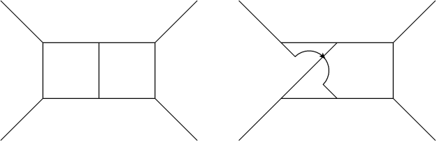
Suppose you’re working with a Yang-Mills theory (not necessarily N=4 super Yang-Mills. To show you the difference between planar and non-planar, I’ll draw some two-loop Feynman diagrams for a process where two particles go in and two particles come out:

planarity1

The diagram on your left is planar, while the diagram on your right is non-planar. The diagram on the left can be written entirely on a flat page (or screen), with no tricks. By contrast, with the diagram on the right I have to cheat and make one of the particle lines jump over another one (that’s what the arrow is meant to show). Try as you might, you can’t twist that diagram so that it lies flat on a plane (at least not while keeping the same particles going in and out). That’s the difference between planar and non-planar.

Now, what does it mean for a theory to be planar or non-planar?

Let’s review some facts about Yang-Mills theories. (For a more detailed explanation, see here). In Yang-Mills there are a certain number of colors, where each one works a bit like a different kind of electric charge. The strong force, the force that holds protons and neutrons together, has three colors, usually referred to as red, blue, and green (this is of course just jargon, not the literal color of the particles).

Forces give rise to particles. In the case of the strong force, those particles are called gluons. Each gluon has a color and an anti-color, where you can think of the color like a positive charge and the anti-color like a negative charge. A given gluon might be red-antiblue, or green-antired, or even red-antired.

While the strong force has three colors, for this article it will be convenient to pretend that there are four: red, green, blue, and yellow.

An important principle of Yang-Mills theories is that color must be conserved. Since anti-colors are like negative colors, they can cancel normal colors out. So if you’ve got a red-antiblue gluon that collides with a blue-antigreen gluon, the blue and antiblue can cancel each other out, and you can end up with, for example, red-antiyellow and yellow-antigreen instead.

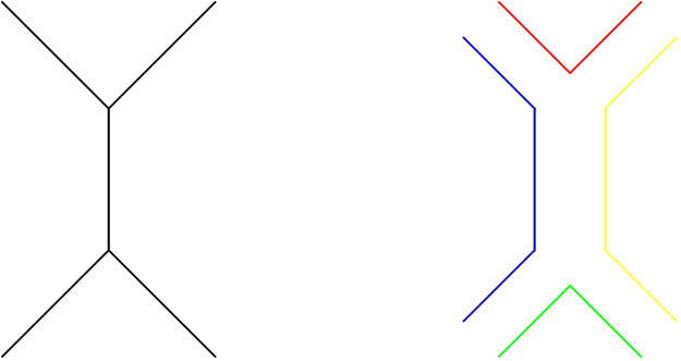
Let’s consider that process in particular. There are lots of Feynman diagrams you can draw for it, let’s draw one of the simplest ones first:

planarity2

The diagram on the left just shows the process in terms of the particles involved: two gluons go in, two come out.

The other diagram takes into account conservation of colors. The red from the red-antiblue gluon becomes the red in the red-antiyellow gluon on the other side. The antiblue instead goes down and meets the blue from the blue-antigreen gluon, and both vanish in the middle, cancelling each other out. It’s as if the blue color entered the diagram, then turned around backwards and left it again. (If you’ve ever heard someone make the crazy-sounding claim that antimatter is normal matter going backwards in time, this is roughly what they mean.)

From this diagram, we can start observing a general principle: to make sure that color is conserved, each line must have only one color.

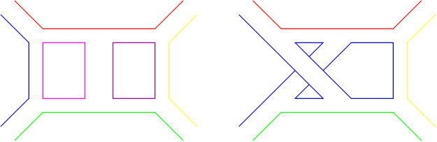
Now let’s try to apply this principle to the two-loop diagrams from the beginning of the article. If you draw double lines like we did in the last example, fill in the colors, and work things out, this is what you get:

planarity3

What’s going on here?

In the diagram on the left, you see the same lines as the earlier diagram on the outside. On the inside, though, I’ve drawn two loops of color, purple and pink.

I drew the lines that way because, just based on the external lines, you don’t know what color they should be. They could be red, or yellow, or green, or blue. Nothing tells you which one is right, so all of them are possible.

Remember that for Feynman diagrams, we need to add up every diagram we can draw to get the final result. That means that there are actually four times four or sixteen copies of this diagram, each one with different colors in the loops.

Now let’s look at the other diagram. Like the first one, it’s a diagram with two loops. However, in this case, the inside of both loops is blue. If you like, you can try to trace out the lines in the loops. You’ll find that they’re all connected together. Because this diagram is non-planar, color conservation fixes the color in the loops.

So while there are sixteen copies of the first diagram, there is only one possible version of the second one. Since you add all the diagrams together, that means that the first diagram is sixteen times more important than the second diagram.

Now suppose we had more than four colors. Lots more.

More than that…

With ten colors, the planar diagrams are a hundred times more important. With a hundred colors, they are ten thousand times more important. Keep increasing the number of colors, and it gets to the point where you can honestly say that the non-planar diagrams don’t matter at all.

What, then, is a “planar theory”?

A planar theory is a theory with a very large (infinite) number of colors.

In a planar theory, you can ignore the non-planar diagrams and focus only on the planar ones.

Nima Arkani-Hamed’s Amplituhedron method applies to the planar version of N=4 super Yang-Mills. There is a lot of progress on the planar version of the theory, and it is because the restriction to planar diagrams makes things simpler.

However, sometimes you need to go beyond planar diagrams. There are relationships between planar and non-planar diagrams, based on the ways that you can pair different colors together in the theory. Fully understanding this relationship is powerful for understanding Yang-Mills theory, but, as it turns out, it’s also the key to relating Yang-Mills theory to gravity! But that’s a story for another post.

The Amplituhedron and Other Excellently Silly Words

15 Replies

Nima Arkani-Hamed recently gave a talk at the Simons Center on the topic of what he and Jaroslav Trnka are calling the Amplituhedron.

There’s an article on it in Quanta Magazine. The article starts out a bit hype-y for my taste (too much language of importance, essentially), but it has several very solid descriptions of the history of the situation. I particularly like how the author concisely describes the Feynman diagram picture in the space of a single paragraph, and I would recommend reading that part even if you don’t have time to read the whole article. In general it’s worth it to get a picture of what’s going on.

That said, I obviously think I can clear a few things up, otherwise I wouldn’t be writing about it, so here I go!

“The” Amplituhedron

Nima’s new construction, the Amplituhedron, encodes amplitudes (building blocks of probabilities in particle physics) in N=4 super Yang-Mills as the “area” of a multi-dimensional analog of a polyhedron (hence, Amplitu-hedron).

Now, I’m a big supporter of silly-sounding words with amplitu- at the beginning (amplitudeologist, anyone?), and this is no exception. Anyway, the word Amplitu-hedron isn’t what’s confusing people. What’s confusing people is the word the.

When the Quanta article says that Nima has found “the” Amplituhedron, it makes it sound like he has discovered one central formula that somehow contains the whole universe. If you read the comments, many readers went away with that impression.

In case you needed me to say it, that’s not what is going on. The problem is in the use of the word “the”.

Suppose it was 1886, and I told you that a fellow named Carl Benz had invented “the Automobile”, a marvelous machine that can get everyone to work on time (as well as become the dominant form of life on Long Island).

My use of “the” might make you imagine that Benz invented some single, giant machine that would roam across the country, picking people up and somehow transporting everyone to work. You’d be skeptical of this, of course, expecting that long queues to use this gigantic, wondrous machine would swiftly ruin any speed advantage it might possess…

The Automobile, here to take you to work.

Or, you could view “the” in another light, as indicating a type of thing.

Much like “the Automobile” is a concept, manifested in many different cars and trucks across the country, “the Amplituhedron” is a concept, manifested in many different amplituhedra, each corresponding to a particular calculation that we might attempt.

Advantages…

Each amplituhedron has to do with an amplitude involving a specific number of particles, with a particular number of internal loops. (The Quanta article has a pretty good explanation of loops, here’s mine if you’d rather read that). Based on the problem you’re trying to solve, there are a set of rules that you use to construct the particular amplituhedron you need. The “area” of this amplituhedron (in quotation marks because I mean the area in an abstract, mathematical sense) is the amplitude for the process, which lets you calculate the probability that whatever particle physics situation you’re describing will happen.

Now, we already have many methods to calculate these probabilities. The amplituhedron’s advantage is that it makes these calculations much simpler. What was once quite a laborious and complicated four-loop calculation, Nima claims can be done by hand using amplituhedra. I didn’t get a chance to ask whether the same efficiency improvement holds true at six loops, but Nima’s description made it sound like it would at least speed things up.

[Edit: Some of my fellow amplitudeologists have reminded me of two things. First, that paper I linked above paved the way to more modern methods for calculating these things, which also let you do the four-loop calculation by hand. (You need only six or so diagrams). Second, even back then the calculation wasn’t exactly “laborious”, there were some pretty slick tricks that sped things up. With that in mind, I’m not sure Nima’s method is faster per se. But it is a fast method that has the other advantages described below.]

The amplituhedron has another, more sociological advantage. By describing the amplitude in terms of a geometrical object rather than in terms of our usual terminology, we phrase things in a way that mathematicians are more likely to understand. By making things more accessible to mathematicians (and the more math-headed physicists), we invite them to help us solve our problems, so that together we can come up with more powerful methods of calculation.

Nima and the Quanta article both make a big deal about how the amplituhedron gets rid of the principles of locality and unitarity, two foundational principles of quantum field theory. I’m a bit more impressed by this than Woit is. The fine distinction that needs to be made here is that the amplituhedron isn’t simply “throwing out” locality and unitarity. Rather, it’s written in such a way that it doesn’t need locality and unitarity to function. In the end, the formulas it computes still obey both principles. Nima’s hope is that, now that we are able to write amplitudes without needing locality and unitarity, if we end up having to throw out either of those principles to make a new theory we will be able to do so. That’s legitimately quite a handy advantage to have, it just doesn’t mean that locality and unitarity must be thrown out right now.

…and Disadvantages

It’s important to remember that this whole story is limited to N=4 super Yang-Mills. Nima doesn’t know how to apply it to other theories, and nobody else seems to have any good ideas either. In addition, this only applies to the planar part of the theory. I’m not going to explain what that term means here; for now just be aware that while there are tricks that let you “square” a calculation in super Yang-Mills to get a similar calculation in quantum gravity, those tricks rely on having non-planar data, or information beyond the planar part of the theory. So at this point, this doesn’t give us any new hints about quantum gravity. It’s conceivable that physicists will find ways around both of these limits, but for now this result, though impressive, is quite limited.

Nima hasn’t found some sort of singular “jewel at the heart of physics”. Rather, he’s found a very slick, very elegant, quite efficient way to make calculations within one particular theory. This is profound, because it expresses things in terms that mathematicians can address, and because it shows that we can write down formulas without relying on what are traditionally some of the most fundamental principles of quantum field theory. Only time will tell whether Nima or others can generalize this picture, taking it beyond planar N=4 super Yang-Mills and into the tougher theories that still await this sort of understanding.

Duality: Find out what it means to me

1 Reply

There’s a cute site out there called Why String Theory. Started by Oxford and the Royal Society, Why String Theory contains lots of concise and well-illustrated explanations of string theory, and it even wades into some of the more complex topics like AdS/CFT and string dualities in general. Their explanation of dualities is a nice introduction to why dualities matter in string theory, but I don’t think it does a very good job of explaining what a duality actually is or how one works. As your fearless host, I’m confident that I can do better.

Why String Theory defines dualities as when “different mathematical theories describe the same physics.” How does that work, though? In what sense are the theories different, if they describe the same thing? And if they describe the same thing, why do we need both of them?

You’ve probably seen the above image before, or one much like it. Look at it one way, and you see a goblet. Another, and you see two faces.

Now imagine that instead of a flat image, these are 3D objects, models you have in your house. You’ve got a goblet, and a pair of clay faces. You’re still pretty sure they fit together like they do in the image, though. Maybe they said they fit together on the packaging, maybe you stuck them together and it didn’t look like there were any gaps. Whatever the reason, you’re confident enough about this that you’re willing to assume it’s true.

Now suppose you want to figure out how long the noses on the faces are. In case you’ve never measured a human nose, I can let you know that it’s tricky. You could put a ruler along the nose, but it would be diagonal rather than straight, so you wouldn’t get an accurate measurement. Even putting the ruler beneath the nose doesn’t work for rounded noses like these.

That said, measuring the goblet is easy. You can run measuring tape around the neck of the goblet to find the circumference, and then calculate the diameter. And if you measure the goblet in this way, you also know how long the faces’ noses are.

You could go further, and build up a list of things you can measure on one object that tell you about the other one. The necks match up to the base of the goblet, the foreheads to the mouth, etc. It would be like a dictionary, translating between two languages: the language of measurements of the faces, and the language of measurements of the goblet.

That sort of “dictionary” is the essence of duality. When two theories have a duality (are dual to each other), you can make a “dictionary” to translate measurements in one theory to measurements in the other. That doesn’t mean, however, that the theories are clearly connected: like 3D models of the faces and the goblet, it may be that without looking at the particular “silhouette” defined by duality the two views are radically different. Rather than physical objects, the theories compare mathematical “objects”, so rather than physical obstructions like the solidity of noses we have to deal with mathematical ones, situations where one quantity or another is easier or harder to calculate depending on how the math is set up. For example, many dualities relate things that require calculations at very high loops to things that can be calculated with fewer loops (for an explanation of loops, check out this post).

As Why String Theory points out, one of the most prominent dualities is called AdS/CFT, and it relates N=4 super Yang-Mills (a Conformal Field Theory, or CFT) to string theory in something called Anti-de Sitter (AdS) space (tricky to describe, but essentially a world in which space is warped like a hyperbola). Another duality relates N=4 super Yang-Mills Feynman diagrams with n particles coming in from outside to diagrams with an n-sided shape and particles randomly coming in from the edges of the shape (these latter diagrams are called Wilson loops). In general N=4 super Yang-Mills is involved in many, many dualities, which is a big part of why it’s so dang cool.

What’s A Graviton? Or: How I Learned to Stop Worrying and Love Quantum Gravity

5 Replies

I’m four gravitons and a grad student. And despite this, I haven’t bothered to explain what a graviton is. It’s time to change that.

Let’s start like we often do, with a quick answer that will take some unpacking:

Gravitons are the force-carrying bosons of gravity.

I mentioned force-carrying bosons briefly here. Basically, a force can either be thought of as a field, or as particles called bosons that carry the effect of that field. Thinking about the force in terms of particles helps, because it allows you to visualize Feynman diagrams. While most forces come from Yang-Mills fields with spin 1, gravity has spin 2.

Now you may well ask, how exactly does this relate to the idea that gravity, unlike other forces, is a result of bending space and time?

First, let’s talk about what it means for space itself to be bent. If space is bent, distances are different than they otherwise would be.

Suppose we’ve got some coordinates: x and y. How do we find a distance? We use the Pythagorean Theorem:

$d^2=x^2+y^2$

Where d is the full distance. If space is bent, the formula changes:

$d^2=g_{x}x^2+g_{y}y^2$

Here $g_{x}$ and $g_{y}$ come from gravity. Normally, they would depend on x and y, modifying the formula and thus “bending” space.

Let’s suppose instead of measuring a distance, we want to measure the momentum of some other particle, which we call $\phi$ because physicists are overly enamored of Greek letters. If $p_{x,\phi}$ is its momentum (physicists also really love subscripts), then its total momentum can be calculated using the Pythagorean Theorem as well:

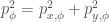
$p_\phi^2= p_{x,\phi}^2+ p_{y,\phi}^2$

Or with gravity:

$p_\phi^2= g_{x}p_{x,\phi}^2+ g_{y} p_{y,\phi}^2$

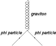
At the moment, this looks just like the distance formula with a bunch of extra stuff in it. Interpreted another way, though, it becomes instructions for the interactions of the graviton. If $g_{x}$ and $g_{y}$ represent the graviton, then this formula says that one graviton can interact with two $\phi$ particles, like so:

Saying that gravitons can interact with $\phi$ particles ends up meaning the same thing as saying that gravity changes the way we measure the $\phi$ particle’s total momentum. This is one of the more important things to understand about quantum gravity: the idea that when people talk about exotic things like “gravitons”, they’re really talking about the same theory that Einstein proposed in 1916. There’s nothing scary about describing gravity in terms of particles just like the other forces. The scary bit comes later, as a result of the particular way that quantum calculations with gravity end up. But that’s a tale for another day.

Nature Abhors a Constant

Why a Quantum Field Theorist is the wrong person to ask about Quantum Mechanics

10 Replies

Quantum Mechanics is quite possibly the sexiest, most mysterious thing to come out of 20^th century physics. Almost a century of evidence has confirmed that the world is fundamentally ambiguous and yet deeply predictable, that physics is best described probabilistically, and that however alien this seems the world wouldn’t work without it. Quantum Mechanics raises deep philosophical questions about the nature of reality, some of the most interesting of which are still unanswered to this day.

And I am (for the moment, at least) not the best person to ask about these questions. Because while I specialize in Quantum Field Theory, that actually means I pay very little attention to the paradoxes of Quantum Mechanics.

It all boils down to the way calculations in quantum field theory work. As I described in a previous post, quantum field theory involves adding up progressively more complicated Feynman Diagrams. There are methods that don’t involve Feynman Diagrams, but in one way or another they work on the same basic principle: to take quantum mechanics into account, add up all possible outcomes, either literally or through shortcuts.

That may sound profound, but in many ways it’s quite mundane. Yes, you’re adding up all possibilities, but each possibility is essentially a mundane possibility. There are a few caveats, but essentially each element you add in, each Feynman Diagram for example, looks roughly like the sort of thing you could get without quantum mechanics.

In a typical quantum field theory calculation, you don’t see the mysterious parts of quantum mechanics: you don’t see entanglement, or measurements collapsing the wavefunction, and you don’t have to think about whether reality is really real. Because of that, I’m not the best person to ask about quantum paradoxes, as I’ve got little more than an undergraduate’s knowledge of these things.

There are people whose work focuses much more on quantum paradoxes. Generally these people focus on systems closer to everyday experiments, atoms rather than more fundamental particles. Because the experimentalists they cooperate with have much more ability to manipulate the systems they study, they are able to probe much more intricate quantum properties. People interested in the possibility of a quantum computer are often at the forefront of this, so if you’ve got a question about a quantum paradox, don’t ask me, ask people like WLOG blog.

A final note: there are many people (often very experienced and elite researchers) who, though they might primarily be described as quantum field theorists, have weighed in on the subject of quantum paradoxes. If you’ve heard of the black hole firewall debate, that is a recent high-profile example of this. The important thing to remember is that these people are masters of many areas of physics. They have taken the time to study the foundations of quantum mechanics, and have broadened their horizons to the tools more commonly used in other subfields. So while your average grad student quantum field theorist won’t know an awful lot about quantum paradoxes, these guys do.

4 gravitons

Stories about physics from someone who's been there