Category Archives: Yang-Mills

Hexagon Functions VI: The Power Cosmic

I have a new paper out this week. It’s the long-awaited companion to a paper I blogged about a few months back, itself the latest step in a program that has made up a major chunk of my research.

The title is a bit of a mouthful, but I’ll walk you through it:

The Cosmic Galois Group and Extended Steinmann Relations for Planar N = 4 SYM Amplitudes

I calculate scattering amplitudes (roughly, probabilities that elementary particles bounce off each other) in a (not realistic, and not meant to be) theory called planar N=4 super-Yang-Mills (SYM for short). I can’t summarize everything we’ve been doing here, but if you read the blog posts I linked above and some of the Handy Handbooks linked at the top of the page you’ll hopefully get a clearer picture.

We started using the Steinmann Relations a few years ago. Discovered in the 60’s, the Steinmann relations restrict the kind of equations we can use to describe particle physics. Essentially, they mean that particles can’t travel two ways at once. In this paper, we extend the Steinmann relations beyond Steinmann’s original idea. We don’t yet know if we can prove this extension works, but it seems to be true for the amplitudes we’re calculating. While we’ve presented this in talks before, this is the first time we’ve published it, and it’s one of the big results of this paper.

The other, more exotic-sounding result, has to do with something called the Cosmic Galois Group.

Évariste Galois, the famously duel-prone mathematician, figured out relations between algebraic numbers (that is, numbers you can get out of algebraic equations) in terms of a mathematical structure called a group. Today, mathematicians are interested not just in algebraic numbers, but in relations between transcendental numbers as well, specifically a kind of transcendental number called a period. These numbers show up a lot in physics, so mathematicians have been thinking about a Galois group for transcendental numbers that show up in physics, a so-called Cosmic Galois Group.

(Cosmic here doesn’t mean it has to do with cosmology. As far as I can tell, mathematicians just thought it sounded cool and physics-y. They also started out with rather ambitious ideas about it, if you want a laugh check out the last few paragraphs of this talk by Cartier.)

For us, Cosmic Galois Theory lets us study the unusual numbers that show up in our calculations. Doing this, we’ve noticed that certain numbers simply don’t show up. For example, the Riemann zeta function shows up often in our results, evaluated at many different numbers…but never evaluated at the number three. Nor does any number related to that one through the Cosmic Galois Group show up. It’s as if the theory only likes some numbers, and not others.

This weird behavior has been observed before. Mathematicians can prove it happens for some simple theories, but it even applies to the theories that describe the real world, for example to calculations of the way an electron’s path is bent by a magnetic field. Each theory seems to have its own preferred family of numbers.

For us, this has been enormously useful. We calculate our amplitudes by guesswork, starting with the right “alphabet” and then filling in different combinations, as if we’re trying all possible answers to a word jumble. Cosmic Galois Theory and Extended Steinmann have enabled us to narrow down our guess dramatically, making it much easier and faster to get to the right answer.

More generally though, we hope to contribute to mathematicians’ investigations of Cosmic Galois Theory. Our examples are more complicated than the simple theories where they currently prove things, and contain more data than the more limited results from electrons. Hopefully together we can figure out why certain numbers show up and others don’t, and find interesting mathematical principles behind the theories that govern fundamental physics.

For now, I’ll leave you with a preview of a talk I’m giving in a couple weeks’ time:

The font, of course, is Cosmic Sans

Hexagon Functions V: Seventh Heaven

I’ve got a new paper out this week, a continuation of a story that has threaded through my career since grad school. With a growing collaboration (now Simon Caron-Huot, Lance Dixon, Falko Dulat, Andrew McLeod, and Georgios Papathanasiou) I’ve been calculating six-particle scattering amplitudes in my favorite theory-that-does-not-describe-the-real-world, N=4 super Yang-Mills. We’ve been pushing to more and more “loops”: tougher and tougher calculations that approximate the full answer better and better, using the “word jumble” trick I talked about in Scientific American. And each time, we learn something new.

Now we’re up to seven loops for some types of particles, and six loops for the rest. In older blog posts I talked in megabytes: half a megabyte for three loops, 15 MB for four loops, 300 MB for five loops. I don’t have a number like that for six and seven loops: we don’t store the result in that way anymore, it just got too cumbersome. We have to store it in a simplified form, and even that takes 80 MB.

Some of what we learned has to do with the types of mathematical functions that we need: our “guess” for the result at each loop. We’ve honed that guess down a lot, and discovered some new simplifications along the way. I won’t tell that story here (except to hint that it has to do with “cosmic Galois theory”) because we haven’t published it yet. It will be out in a companion paper soon.

This paper focused on the next step, going from our guess to the correct six- and seven-loop answers. Here too there were surprises. For the last several loops, we’d observed a surprisingly nice pattern: different configurations of particles with different numbers of loops were related, in a way we didn’t know how to explain. The pattern stuck around at five loops, so we assumed it was the real deal, and guessed the new answer would obey it too.

Yes, in our field this counts as surprisingly nice

Usually when scientists tell this kind of story, the pattern works, it’s a breakthrough, everyone gets a Nobel prize, etc. This time? Nope!

The pattern failed. And it failed in a way that was surprisingly difficult to detect.

The way we calculate these things, we start with a guess and then add what we know. If we know something about how the particles behave at high energies, or when they get close together, we use that to pare down our guess, getting rid of pieces that don’t fit. We kept adding these pieces of information, and each time the pattern seemed ok. It was only when we got far enough into one of these approximations that we noticed a piece that didn’t fit.

That piece was a surprisingly stealthy mathematical function, one that hid from almost every test we could perform. There aren’t any functions like that at lower loops, so we never had to worry about this before. But now, in the rarefied land of six-loop calculations, they finally start to show up.

We have another pattern, like the old one but that isn’t broken yet. But at this point we’re cautious: things get strange as calculations get more complicated, and sometimes the nice simplifications we notice are just accidents. It’s always important to check.

Deep physics or six-loop accident? You decide!

This result was a long time coming. Coordinating a large project with such a widely spread collaboration is difficult, and sometimes frustrating. People get distracted by other projects, they have disagreements about what the paper should say, even scheduling Skype around everyone’s time zones is a challenge. I’m more than a little exhausted, but happy that the paper is out, and that we’re close to finishing the companion paper as well. It’s good to have results that we’ve been hinting at in talks finally out where the community can see them. Maybe they’ll notice something new!


Hexagon Functions Meet the Amplituhedron: Thinking Positive

I finished a new paper recently, it’s up on arXiv now.

This time, we’re collaborating with Jaroslav Trnka, of Amplituhedron fame, to investigate connections between the Amplituhedron and our hexagon function approach.

The Amplituhedron is a way to think about scattering amplitudes in our favorite toy model theory, N=4 super Yang-Mills. Specifically, it describes amplitudes as the “volume” of some geometric space.

Here’s something you might expect: if something is a volume, it should be positive, right? You can’t have a negative amount of space. So you’d naturally guess that these scattering amplitudes, if they’re really the “volume” of something, should be positive.

“Volume” is in quotation marks there for a reason, though, because the real story is a bit more complicated. The Amplituhedron isn’t literally the volume of some space, there are a bunch of other mathematical steps between the geometric story of the Amplituhedron on the one end and the final amplitude on the other. If it was literally a volume, calculating it would be quite a bit easier: mathematicians have gotten very talented at calculating volumes. But if it was literally a volume, it would have to be positive.

What our paper demonstrates is that, in the right regions (selected by the structure of the Amplituhedron), the amplitudes we’ve calculated so far are in fact positive. That first, basic requirement for the amplitude to actually literally be a volume is satisfied.

Of course, this doesn’t prove anything. There’s still a lot of work to do to actually find the thing the amplitude is the volume of, and this isn’t even proof that such a thing exists. It’s another, small piece of evidence. But it’s a reassuring one, and it’s nice to begin to link our approach with the Amplituhedron folks.

This week was the 75th birthday of John Schwarz, one of the founders of string theory and a discoverer of N=4 super Yang-Mills. We’ve dedicated the paper to him. His influence on the field, like the amplitudes of N=4 themselves, has been consistently positive.

Hexagon Functions IV: Steinmann Harder

It’s paper season! I’ve got another paper out this week, this one a continuation of the hexagon function story.

The story so far:

My collaborators and I have been calculating “six-particle” (two particles collide, four come out, or three collide, three come out…) scattering amplitudes (probabilities that particles scatter) in N=4 super Yang-Mills. We calculate them starting with an ansatz (a guess, basically) made up of a type of functions called hexagon functions: “hexagon” because they’re the right functions for six-particle scattering. We then narrow down our guess by bringing in other information: for example, if two particles are close to lining up, our answer needs to match the one calculated with something called the POPE, so we can throw out guesses that don’t match that. In the end, only one guess survives, and we can check that it’s the right answer.

So what’s new this time?

More loops:

In quantum field theory, most of our calculations are approximate, and we measure the precision in something called loops. The more loops, the closer we are to the exact result, and the more complicated the calculation becomes.

This time, we’re at five loops of precision. To give you an idea of how complicated that is: I store these functions in text files. We’ve got a new, more efficient notation for them. With that, the two-loop functions fit into files around 20KB. Three loops, 500KB. Four, 15MB. And five? 300MB.

So if you want to imagine five loops, think about something that needs to be stored in a 300MB text file.

More insight:

We started out having noticed some weird new symmetries of our old results, so we brought in Simon Caron-Huot, expert on weird new symmetries. He couldn’t figure out that one…but he did notice an entirely different symmetry, one that turned out to have been first noticed in the 60’s, called the Steinmann relations.

The core idea of the Steinmann relations goes back to the old method of calculating amplitudes, with Feynman diagrams. In Feynman diagrams, lines represent particles traveling from one part of the diagram to the other. In a simplified form, the Steinmann conditions are telling us that diagrams can’t take two mutually exclusive shapes at the same time. If three particles are going one way, they can’t also be going another way.

steinmann2

With the Steinmann relations, things suddenly became a whole lot easier. Calculations that we had taken months to do, Simon was now doing in a week. Finally we could narrow things down and get the full answer, and we could do it with clear, physics-based rules.

More bootstrap:

In physics, when we call something a “bootstrap” it’s in reference to the phrase “pull yourself up by your own boostraps”. That impossible task, lifting yourself  with no outside support, is essentially what we do when we “bootstrap”: we do a calculation with no external input, simply by applying general rules.

In the past, our hexagon function calculations always had some sort of external data. For the first time, with the Steinmann conditions, we don’t need that. Every constraint, everything we do to narrow down our guess, is either a general rule or comes out of our lower-loop results. We never need detailed information from anywhere else.

This is big, because it might allow us to avoid loops altogether. Normally, each loop is an approximation, narrowed down using similar approximations from others. If we don’t need the approximations from others, though, then we might not need any approximations at all. For this particular theory, for this toy model, we might be able to actually calculate scattering amplitudes exactly, for any strength of forces and any energy. Nobody’s been able to do that for this kind of theory before.

We’re already making progress. We’ve got some test cases, simpler quantities that we can understand with no approximations. We’re starting to understand the tools we need, the pieces of our bootstrap. We’ve got a real chance, now, of doing something really fundamentally new.

So keep watching this blog, keep your eyes on arXiv: big things are coming.

The “Lies to Children” Model of Science Communication, and The “Amplitudes Are Weird” Model of Amplitudes

Let me tell you a secret.

Scattering amplitudes in N=4 super Yang-Mills don’t actually make sense.

Scattering amplitudes calculate the probability that particles “scatter”: coming in from far away, interacting in some fashion, and producing new particles that travel far away in turn. N=4 super Yang-Mills is my favorite theory to work with: a highly symmetric version of the theory that describes the strong nuclear force. In particular, N=4 super Yang-Mills has conformal symmetry: if you re-scale everything larger or smaller, you should end up with the same predictions.

You might already see the contradiction here: scattering amplitudes talk about particles coming in from very far away…but due to conformal symmetry, “far away” doesn’t mean anything, since we can always re-scale it until it’s not far away anymore!

So when I say that I study scattering amplitudes in N=4 super Yang-Mills, am I lying?

Well…yes. But it’s a useful type of lie.

There’s a concept in science writing called “lies to children”, first popularized in a fantasy novel.

the-science-of-discworld-1

This one.

When you explain science to the public, it’s almost always impossible to explain everything accurately. So much background is needed to really understand most of modern science that conveying even a fraction of it would bore the average audience to tears. Instead, you need to simplify, to skip steps, and even (to be honest) to lie.

The important thing to realize here is that “lies to children” aren’t meant to mislead. Rather, they’re chosen in such a way that they give roughly the right impression, even as they leave important details out. When they told you in school that energy is always conserved, that was a lie: energy is a consequence of symmetry in time, and when that symmetry is broken energy doesn’t have to be conserved. But “energy is conserved” is a useful enough rule that lets you understand most of everyday life.

In this case, the “lie” that we’re calculating scattering amplitudes is fairly close to the truth. We’re using the same methods that people use to calculate scattering amplitudes in theories where they do make sense, like QCD. For a while, people thought these scattering amplitudes would have to be zero, since anything else “wouldn’t make sense”…but in practice, we found they were remarkably similar to scattering amplitudes in other theories. Now, we have more rigorous definitions for what we’re calculating that avoid this problem, involving objects called polygonal Wilson loops.

This illustrates another principle, one that hasn’t (yet) been popularized by a fantasy novel. I’d like to call it the “amplitudes are weird” principle. Time and again we amplitudes-folks will do a calculation that doesn’t really make sense, find unexpected structure, and go back to figure out what that structure actually means. It’s been one of the defining traits of the field, and we’ve got a pretty good track record with it.

A couple of weeks back, Lance Dixon gave an interview for the SLAC website, talking about his work on quantum gravity. This was immediately jumped on by Peter Woit and Lubos Motl as ammo for the long-simmering string wars. To one extent or another, both tried to read scientific arguments into the piece. This is in general a mistake: it is in the nature of a popularization piece to contain some volume of lies-to-children, and reading a piece aimed at a lower audience can be just as confusing as reading one aimed at a higher audience.

In the remainder of this post, I’ll try to explain what Lance was talking about in a slightly higher-level way. There will still be lies-t0-children involved, this is a popularization blog after all. But I should be able to clear up a few misunderstandings. Lubos probably still won’t agree with the resulting argument, but it isn’t the self-evidently wrong one he seems to think it is.

Lance Dixon has done a lot of work on quantum gravity. Those of you who’ve read my old posts might remember that quantum gravity is not so difficult in principle: general relativity naturally leads you to particles called gravitons, which can be treated just like other particles. The catch is that the theory that you get by doing this fails to be predictive: one reason why is that you get an infinite number of erroneous infinite results, which have to be papered over with an infinite number of arbitrary constants.

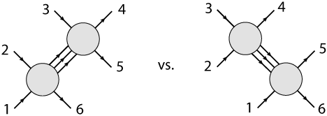
Working with these non-predictive theories, however, can still yield interesting results. In the article, Lance mentions the work of Bern, Carrasco, and Johansson. BCJ (as they are abbreviated) have found that calculating a gravity amplitude often just amounts to calculating a (much easier to find) Yang-Mills amplitude, and then squaring the right parts. This was originally found in the context of string theory by another three-letter group, Kawai, Lewellen, and Tye (or KLT). In string theory, it’s particularly easy to see how this works, as it’s a basic feature of how string theory represents gravity. However, the string theory relations don’t tell the whole story: in particular, they only show that this squaring procedure makes sense on a classical level. Once quantum corrections come in, there’s no known reason why this squaring trick should continue to work in non-string theories, and yet so far it has. It would be great if we had a good argument why this trick should continue to work, a proof based on string theory or otherwise: for one, it would allow us to be much more confident that our hard work trying to apply this trick will pay off! But at the moment, this falls solidly under the “amplitudes are weird” principle.

Using this trick, BCJ and collaborators (frequently including Lance Dixon) have been calculating amplitudes in N=8 supergravity, a highly symmetric version of those naive, non-predictive gravity theories. For this particular, theory, the theory you “square” for the above trick is N=4 super Yang-Mills. N=4 super Yang-Mills is special for a number of reasons, but one is that the sorts of infinite results that lose you predictive power in most other quantum field theories never come up. Remarkably, the same appears to be true of N=8 supergravity. We’re still not sure, the relevant calculation is still a bit beyond what we’re capable of. But in example after example, N=8 supergravity seems to be behaving similarly to N=4 super Yang-Mills, and not like people would have predicted from its gravitational nature. Once again, amplitudes are weird, in a way that string theory helped us discover but by no means conclusively predicted.

If N=8 supergravity doesn’t lose predictive power in this way, does that mean it could describe our world?

In a word, no. I’m not claiming that, and Lance isn’t claiming that. N=8 supergravity simply doesn’t have the right sorts of freedom to give you something like the real world, no matter how you twist it. You need a broader toolset (string theory generally) to get something realistic. The reason why we’re interested in N=8 supergravity is not because it’s a candidate for a real-world theory of quantum gravity. Rather, it’s because it tells us something about where the sorts of dangerous infinities that appear in quantum gravity theories really come from.

That’s what’s going on in the more recent paper that Lance mentioned. There, they’re not working with a supersymmetric theory, but with the naive theory you’d get from just trying to do quantum gravity based on Einstein’s equations. What they found was that the infinity you get is in a certain sense arbitrary. You can’t get rid of it, but you can shift it around (infinity times some adjustable constant 😉 ) by changing the theory in ways that aren’t physically meaningful. What this suggests is that, in a sense that hadn’t been previously appreciated, the infinite results naive gravity theories give you are arbitrary.

The inevitable question, though, is why would anyone muck around with this sort of thing when they could just use string theory? String theory never has any of these extra infinities, that’s one of its most important selling points. If we already have a perfectly good theory of quantum gravity, why mess with wrong ones?

Here, Lance’s answer dips into lies-to-children territory. In particular, Lance brings up the landscape problem: the fact that there are 10^500 configurations of string theory that might loosely resemble our world, and no clear way to sift through them to make predictions about the one we actually live in.

This is a real problem, but I wouldn’t think of it as the primary motivation here. Rather, it gets at a story people have heard before while giving the feeling of a broader issue: that string theory feels excessive.

princess_diana_wedding_dress

Why does this have a Wikipedia article?

Think of string theory like an enormous piece of fabric, and quantum gravity like a dress. You can definitely wrap that fabric around, pin it in the right places, and get a dress. You can in fact get any number of dresses, elaborate trains and frilly togas and all sorts of things. You have to do something with the extra material, though, find some tricky but not impossible stitching that keeps it out of the way, and you have a fair number of choices of how to do this.

From this perspective, naive quantum gravity theories are things that don’t qualify as dresses at all, scarves and socks and so forth. You can try stretching them, but it’s going to be pretty obvious you’re not really wearing a dress.

What we amplitudes-folks are looking for is more like a pencil skirt. We’re trying to figure out the minimal theory that covers the divergences, the minimal dress that preserves modesty. It would be a dress that fits the form underneath it, so we need to understand that form: the infinities that quantum gravity “wants” to give rise to, and what it takes to cancel them out. A pencil skirt is still inconvenient, it’s hard to sit down for example, something that can be solved by adding extra material that allows it to bend more. Similarly, fixing these infinities is unlikely to be the full story, there are things called non-perturbative effects that probably won’t be cured. But finding the minimal pencil skirt is still going to tell us something that just pinning a vast stretch of fabric wouldn’t.

This is where “amplitudes are weird” comes in in full force. We’ve observed, repeatedly, that amplitudes in gravity theories have unexpected properties, traits that still aren’t straightforwardly explicable from the perspective of string theory. In our line of work, that’s usually a sign that we’re on the right track. If you’re a fan of the amplituhedron, the project here is along very similar lines: both are taking the results of plodding, not especially deep loop-by-loop calculations, observing novel simplifications, and asking the inevitable question: what does this mean?

That far-term perspective, looking off into the distance at possible insights about space and time, isn’t my style. (It isn’t usually Lance’s either.) But for the times that you want to tell that kind of story…well, this isn’t that outlandish of a story to tell. And unless your primary concern is whether a piece gives succor to the Woits of the world, it shouldn’t be an objectionable one.

Hexagon Functions III: Now with More Symmetry

I’ve got a new paper up this week.

It’s a continuation of my previous work, understanding collisions involving six particles in my favorite theory, N=4 super Yang-Mills.

This time, we’re pushing up the complexity, going from three “loops” to four. In the past, I could have impressed you with the number of pages the formulas I’m calculating take up (eight hundred pages for the three-loop formula from that first Hexagon Functions paper). Now, though, I don’t have that number: putting my four-loop formula into a pdf-making program just crashes the program. Instead, I’ll have to impress you with file sizes: 2.6 MB for the three-loop formula, 96 MB for the four-loop one.

Calculating such a formula sounds like a pretty big task, and it was, the first time. But things got a lot simpler after a chat I had at Amplitudes.

We calculate these things using an ansatz, a guess for what the final answer should look like. The more vague our guess, the more parameters we need to fix, and the more work we have in general. If we can guess more precisely, we can start with fewer parameters and things are a lot easier.

Often, more precise guesses come from understanding the symmetries of the problem. If we can know that the final answer must be the same after making some change, we can rule out a lot of possibilities.

Sometimes, these symmetries are known features of the answer, things that someone proved had to be correct. Other times, though, they’re just observations, things that have been true in the past and might be true again.

We started out using an observation from three loops. That got us pretty far, but we still had a lot of work to do: 808 parameters, to be fixed by other means. Fixing them took months of work, and throughout we hoped that there was some deeper reason behind the symmetries we observed.

Finally, at Amplitudes, I ran into fellow amplitudeologist Simon Caron-Huot and asked him if he knew the source of our observed symmetry. In just a few days he was able to link it to supersymmetry, giving us justification for our jury rigged trick. However, we figured out that his explanation went further than any of us expected. In the end, rather than 808 parameters we only really needed to consider 34.

Thirty-four options to consider. Thirty-four possible contributions to a ~100 MB file. That might not sound like a big deal, but compared to eight hundred and eight it’s a huge deal. More symmetry means easier calculations, meaning we can go further. At this point going to the next step in complexity, to five loops rather than four, might be well within reach.

Hexagon Functions II: Lost in (super)Space

My new paper went up last night.

It’s on a very similar topic to my last paper, actually. That paper dealt with a specific process involving six particles in my favorite theory, N=4 super Yang-Mills. Two particles collide, and after the metaphorical dust settles four particles emerge. That means six “total” particles, if you add the two in with the four out, for a “hexagon” of variables. To understand situations like that, my collaborators and I created “hexagon functions”, formulas that depended on the states of the six particles.

One thing I didn’t emphasize then was that that calculation only applied to one specific choice of particles, one in which all of the particles are Yang-Mills bosons, particles (like photons) created by the fundamental forces. There are lots of other particles in N=4 super Yang-Mills, though. What happens when they collide?

That question is answered by my new paper. Though it may sound surprising, all of the other particles can be taken into account with a single formula. In order to explain why, I have to tell you about something called superspace.

A while back I complained about a blog post by George Musser about the (2,0) theory. One of the things that irked me about that post was his attempt to explain superspace:

Supersymmetry is the idea that spacetime, in addition to its usual dimensions of space and time, has an entirely different type of dimension—a quantum dimension, whose coordinates are not ordinary real numbers but a whole new class of number that can be thought of as the square roots of zero.

This is actually a great way to think about superspace…if you’re already a physicist. If you’re not, it’s not very informative. Here’s a better way to think about it:

As I’ve talked about before, supersymmetry is a relationship between different types of particles. Two particles related by supersymmetry have the same mass, and the same charge. While they can be very different in other ways (specifically, having different spin), supersymmetric particles are described by many of the same equations as each-other. Rather than writing out those equations multiple times, it’s often nicer to write them all in a unified way, and that’s where superspace comes in.

At its simplest, superspace is just a trick used to write equations in a simpler way. Instead of writing down a different equation for each particle we write one equation with an extra variable, representing a “dimension” of supersymmetry. Traveling in that dimension takes you from particle to particle, in the same way that “turning” the theory (as I phrase it here) does, but it does it within the space of a single equation.

That, essentially, is the trick that we use. With four “superspace dimensions”, we can include the four supersymmetries of N=4 super Yang-Mills, showing how the formulas vary when you go beyond the equation from our first paper.

So far, you may be wondering why I’m calling superspace a “dimension”, when it probably sounds like more of a label. I’ve mentioned before that, just because something is a variable, doesn’t mean it counts as a real dimension.

The key difference is that superspace dimensions are related to regular dimensions in a precise way. In a sense, they’re the square roots of regular dimensions. (Though independently, as George Musser described, they’re the square roots of zero: go in the same direction twice in supersymmetry, and you get back where you’re started, going zero distance.) The coexistence of these two seemingly contradictory statements isn’t some sort of quantum mystery, it’s just a consequence of the fact that, mathematically, I’m saying two very different things. I just can’t think of a way to explain them differently without math.

Superspace isn’t a real place…but it can often be useful to think of it that way. In theories with supersymmetry, it can unify the world, putting disparate particles together into a single equation.

Gravity is Yang-Mills Squared

There’s a concept that I’ve wanted to present for quite some time. It’s one of the coolest accomplishments in my subfield, but I thought that explaining it would involve too much technical detail. However, the recent BICEP2 results have brought one aspect of it to the public eye, so I’ve decided that people are ready.

If you’ve been following the recent announcements by the BICEP2 telescope of their indirect observation of primordial gravitational waves, you’ve probably seen the phrases “E-mode polarization” and “B-mode polarization” thrown around. You may even have seen pictures, showing that light in the cosmic microwave background is polarized differently by quantum fluctuations in the inflaton field and by quantum fluctuations in gravity.

But why is there a difference? What’s unique about gravitational waves that makes them different from the other waves in nature?

As it turns out, the difference all boils down to one statement:

Gravity is Yang-Mills squared.

This is both a very simple claim and a very subtle one, and it comes up in many many places in physics.

Yang-Mills, for those who haven’t read my older posts, is a general category that contains most of the fundamental forces. Electromagnetism, the strong nuclear force, and the weak nuclear force are all variants of Yang-Mills forces.

Yang-Mills forces have “spin 1”. Another way to say this is that Yang-Mills forces are vector forces. If you remember vectors from math class, you might remember that a vector has a direction and a strength. This hopefully makes sense: forces point in a direction, and have a strength. You may also remember that vectors can also be described in terms of components. A vector in four space-time dimensions has four components: x, y, z, and time, like so:

\left( \begin{array}{c} x \\ y \\ z \\ t \end{array} \right)

Gravity has “spin 2”.

As I’ve talked about before, gravity bends space and time, which means that it modifies the way you calculate distances. In practice, that means it needs to be something that can couple two vectors together: a matrix, or more precisely, a tensor, like so:

\left( \begin{array}{cccc} xx & xy & xz & xt\\ yx & yy & yz & yt\\ zx & zy & zz & zt\\ tx & ty & tz & tt\end{array} \right)

So while a Yang-Mills force has four components, gravity has sixteen. Gravity is Yang-Mills squared.

(Technical note: gravity actually doesn’t use all sixteen components, because it’s traceless and symmetric. However, often when studying gravity’s quantum properties theorists often add on extra fields to “complete the square” and fill in the remaining components.)

There’s much more to the connection than that, though. For one, it appears in the kinds of waves the two types of forces can create.

In order to create an electromagnetic wave you need a dipole, a negative charge and a positive charge at opposite ends of a line, and you need that dipole to change over time.

Change over time, of course, is a property of Gifs.

Gravity doesn’t have negative and positive charges, it just has one type of charge. Thus, to create gravitational waves you need not a dipole, but a quadrupole: instead of a line between two opposite charges, you have four gravitational charges (masses) arranged in a square. This creates a “breathing” sort of motion, instead of the back-and-forth motion of electromagnetic waves.

This is your brain on gravitational waves.

This is why gravitational waves have a different shape than electromagnetic waves, and why they have a unique effect on the cosmic microwave background, allowing them to be spotted by BICEP2. Gravity, once again, is Yang-Mills squared.

But wait there’s more!

So far, I’ve shown you that gravity is the square of Yang-Mills, but not in a very literal way. Yes, there are lots of similarities, but it’s not like you can just square a calculation in Yang-Mills and get a calculation in gravity, right?

Well actually…

In quantum field theory, calculations are traditionally done using tools called Feynman diagrams, organized by how many loops the diagram contains. The simplest diagrams have no loops, and are called tree diagrams.

Fascinatingly, for tree diagrams the message of this post is as literal as it can be. Using something called the Kawai-Lewellen-Tye relations, the result of a tree diagram calculation in gravity can be found just by taking a similar calculation in Yang-Mills and squaring it.

(Interestingly enough, these relations were originally discovered using string theory, but they don’t require string theory to work. It’s yet another example of how string theory functions as a laboratory to make discoveries about quantum field theory.)

Does this hold beyond tree diagrams? As it turns out, the answer is again yes!
The calculation involved is a little more complicated, but as discovered by Zvi Bern, John Joseph Carrasco, and Henrik Johansson, if you can get your calculation in Yang-Mills into the right format then all you need to do is square the right thing at the right step to get gravity, even for diagrams with loops!

zvi-bern-350

carrasco

This trick, called BCJ duality after its discoverers, has allowed calculations in quantum gravity that far outpace what would be possible without it. In N=8 supergravity, the gravity analogue of N=4 super Yang-Mills, calculations have progressed up to four loops, and have revealed tantalizing hints that the uncontrolled infinities that usually plague gravity theories are absent in N=8 supergravity, even without adding in string theory. Results like these are why BCJ duality is viewed as one of the “foundational miracles” of the field for those of us who study scattering amplitudes.

Gravity is Yang-Mills squared, in more ways than one. And because gravity is Yang-Mills squared, gravity may just be tame-able after all.

Update on the Amplituhedron

Awhile back I wrote a post on the Amplituhedron, a type of mathematical object  found by Nima Arkani-Hamed and Jaroslav Trnka that can be used to do calculations of scattering amplitudes in planar N=4 super Yang-Mills theory. (Scattering amplitudes are formulas used to calculate probabilities in particle physics, from the probability that an unstable particle will decay to the probability that a new particle could be produced by a collider.) Since then, they published two papers on the topic, the most recent of which came out the day before New Year’s Eve. These papers laid out the amplituhedron concept in some detail, and answered a few lingering questions. The latest paper focused on one particular formula, the probability that two particles bounce off each other. In discussing this case, the paper serves two purposes:

1. Demonstrating that Arkani-Hamed and Trnka did their homework.

2. Showing some advantages of the amplituhedron setup.

Let’s talk about them one at a time.

Doing their homework

There’s already a lot known about N=4 super Yang-Mills theory. In order to propose a new framework like the amplituhedron, Arkani-Hamed and Trnka need to show that the new framework can reproduce the old knowledge. Most of the paper is dedicated to doing just that. In several sections Arkani-Hamed and Trnka show that the amplituhedron reproduces known properties of the amplitude, like the behavior of its logarithm, its collinear limit (the situation when two momenta in the calculation become parallel), and, of course, unitarity.

What, you heard the amplituhedron “removes” unitarity? How did unitarity get back in here?

This is something that has confused several commenters, both here and on Ars Technica, so it bears some explanation.

Unitarity is the principle that enforces the laws of probability. In its simplest form, unitarity requires that all probabilities for all possible events add up to one. If this seems like a pretty basic and essential principle, it is! However, it and locality (the idea that there is no true “action at a distance”, that particles must meet to interact) can be problematic, causing paradoxes for some approaches to quantum gravity. Paradoxes like these inspired Arkani-Hamed to look for ways to calculate scattering amplitudes that don’t rely on locality and unitarity, and with the amplituhedron he succeeded.

However, just because the amplituhedron doesn’t rely on unitarity and locality, doesn’t mean it violates them. The amplituhedron, for all its novelty, still calculates quantities in N=4 super Yang-Mills. N=4 super Yang-Mills is well understood, it’s well-behaved and cuddly, and it obeys locality and unitarity.

This is why the amplituhedron is not nearly as exciting as a non-physicist might think. The amplituhedron, unlike most older methods, isn’t based on unitarity and locality. However, the final product still has to obey unitarity and locality, because it’s the same final product that others calculate through other means. So it’s not as if we’ve completely given up on basic principles of physics.

Not relying on unitarity and locality is valuable. For those who research scattering amplitudes, it has often been useful to try to “eliminate” one principle or another from our calculations. 20 years ago, avoiding Feynman diagrams was the key to finding dramatic simplifications. Now, many different approaches try to sidestep different principles. (For example, while the amplituhedron calculates an integrand and leaves a final integral to be done, I’m working on approaches that never employ an integrand.)

If we can avoid relying on some “basic” principle, that’s usually good evidence that the principle might be a consequence of something even more basic. By showing how unitarity can arise from the amplituhedron, Arkani-Hamed and Trnka have shown that a seemingly basic principle can come out of a theory that doesn’t impose it.

Advantages of the Amplituhedron

Not all of the paper compares to old results and principles, though. A few sections instead investigate novel territory, and in doing so show some of the advantages and disadvantages of the amplituhedron.

Last time I wrote on this topic, I was unclear on whether the amplituhedron was more efficient than existing methods. At this point, it appears that it is not. While the formula that the amplituhedron computes has been found by other methods up to seven loops, the amplituhedron itself can only get up to three loops or so in practical cases. (Loops are a way that calculations are classified in particle physics. More loops means a more complex calculation, and a more precise final result.)

The amplituhedron’s primary advantage is not in efficiency, but rather in the fact that its mathematical setup makes it straightforward to derive interesting properties for any number of loops desired. As Trnka occasionally puts it, the central accomplishment of the amplituhedron is to find “the question to which the amplitude is the answer”. By being able to phrase this “question” mathematically, one can be very general, which allows them to discover several properties that should hold no matter how complex the rest of the calculation becomes. It also has another implication: if this mathematical question has a complete mathematical answer, that answer could calculate the amplitude for any number of loops. So while the amplituhedron is not more efficient than other methods now, it has the potential to be dramatically more efficient if it can be fully understood.

All that said, it’s important to remember that the amplituhedron is still limited in scope. Currently, it applies to a particular theory, one that doesn’t (and isn’t meant to) describe the real world. It’s still too early to tell whether similar concepts can be defined for more realistic theories. If they can, though, it won’t depend on supersymmetry or string theory. One of the most powerful techniques for making predictions for the Large Hadron Collider, the technique of generalized unitarity, was first applied to N=4 super Yang-Mills. While the amplituhedron is limited now, I would not be surprised if it (and its competitors) give rise to practical techniques ten or twenty years down the line. It’s happened before, after all.

Planar vs. Non-Planar: A Colorful Story

Last week, I used two terms, planar theory and non-planar theory, without defining them. This week, I’m going to explain what they mean, and why they’re important.

Suppose you’re working with a Yang-Mills theory (not necessarily N=4 super Yang-Mills. To show you the difference between planar and non-planar, I’ll draw some two-loop Feynman diagrams for a process where two particles go in and two particles come out:

planarity1

The diagram on your left is planar, while the diagram on your right is non-planar. The diagram on the left can be written entirely on a flat page (or screen), with no tricks. By contrast, with the diagram on the right I have to cheat and make one of the particle lines jump over another one (that’s what the arrow is meant to show). Try as you might, you can’t twist that diagram so that it lies flat on a plane (at least not while keeping the same particles going in and out). That’s the difference between planar and non-planar.

Now, what does it mean for a theory to be planar or non-planar?

Let’s review some facts about Yang-Mills theories. (For a more detailed explanation, see here). In Yang-Mills there are a certain number of colors, where each one works a bit like a different kind of electric charge. The strong force, the force that holds protons and neutrons together, has three colors, usually referred to as red, blue, and green (this is of course just jargon, not the literal color of the particles).

Forces give rise to particles. In the case of the strong force, those particles are called gluons. Each gluon has a color and an anti-color, where you can think of the color like a positive charge and the anti-color like a negative charge. A given gluon might be red-antiblue, or green-antired, or even red-antired.

While the strong force has three colors, for this article it will be convenient to pretend that there are four: red, green, blue, and yellow.

An important principle of Yang-Mills theories is that color must be conserved. Since anti-colors are like negative colors, they can cancel normal colors out. So if you’ve got a red-antiblue gluon that collides with a blue-antigreen gluon, the blue and antiblue can cancel each other out, and you can end up with, for example, red-antiyellow and yellow-antigreen instead.

Let’s consider that process in particular. There are lots of Feynman diagrams you can draw for it, let’s draw one of the simplest ones first:

planarity2

The diagram on the left just shows the process in terms of the particles involved: two gluons go in, two come out.

The other diagram takes into account conservation of colors. The red from the red-antiblue gluon becomes the red in the red-antiyellow gluon on the other side. The antiblue instead goes down and meets the blue from the blue-antigreen gluon, and both vanish in the middle, cancelling each other out. It’s as if the blue color entered the diagram, then turned around backwards and left it again. (If you’ve ever heard someone make the crazy-sounding claim that antimatter is normal matter going backwards in time, this is roughly what they mean.)

From this diagram, we can start observing a general principle: to make sure that color is conserved, each line must have only one color.

Now let’s try to apply this principle to the two-loop diagrams from the beginning of the article. If you draw double lines like we did in the last example, fill in the colors, and work things out, this is what you get:

planarity3

What’s going on here?

In the diagram on the left, you see the same lines as the earlier diagram on the outside. On the inside, though, I’ve drawn two loops of color, purple and pink.

I drew the lines that way because, just based on the external lines, you don’t know what color they should be. They could be red, or yellow, or green, or blue. Nothing tells you which one is right, so all of them are possible.

Remember that for Feynman diagrams, we need to add up every diagram we can draw to get the final result. That means that there are actually four times four or sixteen copies of this diagram, each one with different colors in the loops.

Now let’s look at the other diagram. Like the first one, it’s a diagram with two loops. However, in this case, the inside of both loops is blue. If you like, you can try to trace out the lines in the loops. You’ll find that they’re all connected together. Because this diagram is non-planar, color conservation fixes the color in the loops.

So while there are sixteen copies of the first diagram, there is only one possible version of the second one. Since you add all the diagrams together, that means that the first diagram is sixteen times more important than the second diagram.

Now suppose we had more than four colors. Lots more.

More than that…

With ten colors, the planar diagrams are a hundred times more important. With a hundred colors, they are ten thousand times more important. Keep increasing the number of colors, and it gets to the point where you can honestly say that the non-planar diagrams don’t matter at all.

What, then, is a “planar theory”?

A planar theory is a theory with a very large (infinite) number of colors.

In a planar theory, you can ignore the non-planar diagrams and focus only on the planar ones.

Nima Arkani-Hamed’s Amplituhedron method applies to the planar version of N=4 super Yang-Mills. There is a lot of progress on the planar version of the theory, and it is because the restriction to planar diagrams makes things simpler.

However, sometimes you need to go beyond planar diagrams. There are relationships between planar and non-planar diagrams, based on the ways that you can pair different colors together in the theory. Fully understanding this relationship is powerful for understanding Yang-Mills theory, but, as it turns out, it’s also the key to relating Yang-Mills theory to gravity! But that’s a story for another post.