Path Integrals and Loop Integrals: Different Things!

9 Replies

When talking science, we need to be careful with our words. It’s easy for people to see a familiar word and assume something totally different from what we intend. And if we use the same word twice, for two different things…

I’ve noticed this problem with the word “integral”. When physicists talk about particle physics, there are two kinds of integrals we mention: path integrals, and loop integrals. I’ve seen plenty of people get confused, and assume that these two are the same thing. They’re not, and it’s worth spending some time explaining the difference.

Let’s start with path integrals (also referred to as functional integrals, or Feynman integrals). Feynman promoted a picture of quantum mechanics in which a particle travels along many different paths, from point A to point B.

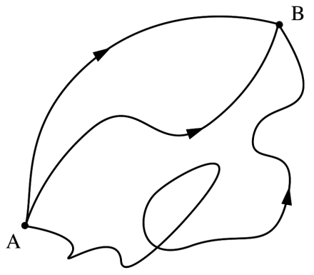
You’ve probably seen a picture like this. Classically, a particle would just take one path, the shortest path, from A to B. In quantum mechanics, you have to add up all possible paths. Most longer paths cancel, so on average the short, classical path is the most important one, but the others do contribute, and have observable, quantum effects. The sum over all paths is what we call a path integral.

It’s easy enough to draw this picture for a single particle. When we do particle physics, though, we aren’t usually interested in just one particle: we want to look at a bunch of different quantum fields, and figure out how they will interact.

We still use a path integral to do that, but it doesn’t look like a bunch of lines from point A to B, and there isn’t a convenient image I can steal from Wikipedia for it. The quantum field theory path integral adds up, not all the paths a particle can travel, but all the ways a set of quantum fields can interact.

How do we actually calculate that?

One way is with Feynman diagrams, and (often, but not always) loop integrals.

4grav2loop

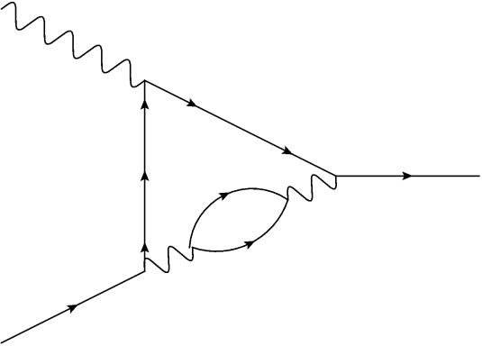
I’ve talked about Feynman diagrams before. Each one is a picture of one possible way that particles can travel, or that quantum fields can interact. In some (loose) sense, each one is a single path in the path integral.

Each diagram serves as instructions for a calculation. We take information about the particles, their momenta and energy, and end up with a number. To calculate a path integral exactly, we’d have to add up all the diagrams we could possibly draw, to get a sum over all possible paths.

(There are ways to avoid this in special cases, which I’m not going to go into here.)

Sometimes, getting a number out of a diagram is fairly simple. If the diagram has no closed loops in it (if it’s what we call a tree diagram) then knowing the properties of the in-coming and out-going particles is enough to know the rest. If there are loops, though, there’s uncertainty: you have to add up every possible momentum of the particles in the loops. You do that with a different integral, and that’s the one that we sometimes refer to as a loop integral. (Perhaps confusingly, these are also often called Feynman integrals: Feynman did a lot of stuff!)

$\frac{i^{a+l(1-d/2)}\pi^{ld/2}}{\prod_i \Gamma(a_i)}\int_0^\infty...\int_0^\infty \prod_i\alpha_i^{a_i-1}U^{-d/2}e^{iF/U-i\sum m_i^2\alpha_i}d\alpha_1...d\alpha_n$

Loop integrals can be pretty complicated, but at heart they’re the same sort of thing you might have seen in a calculus class. Mathematicians are pretty comfortable with them, and they give rise to numbers that mathematicians find very interesting.

Path integrals are very different. In some sense, they’re an “integral over integrals”, adding up every loop integral you could write down. Mathematicians can define path integrals in special cases, but it’s still not clear that the general case, the overall path integral picture we use, actually makes rigorous mathematical sense.

So if you see physicists talking about integrals, it’s worth taking a moment to figure out which one we mean. Path integrals and loop integrals are both important, but they’re very, very different things.

We Didn’t Deserve Hawking

9 Replies

I don’t usually do obituaries. I didn’t do one when Joseph Polchinksi died, though his textbook is sitting an arm’s reach from me right now. I never collaborated with Polchinski, I never met him, and others were much better at telling his story.

I never met Stephen Hawking, either. When I was at Perimeter, I’d often get asked if I had. Visitors would see his name on the Perimeter website, and I’d have to disappoint them by explaining that he hadn’t visited the institute in quite some time. His health, while exceptional for a septuagenarian with ALS, wasn’t up to the travel.

Was his work especially relevant to mine? Only because of its relevance to everyone who does gravitational physics. The universality of singularities in general relativity, black hole thermodynamics and Hawking radiation, these sharpened the questions around quantum gravity. Without his work, string theory wouldn’t have tried to answer the questions Hawking posed, and it wouldn’t have become the field it is today.

Hawking was unique, though, not necessarily because of his work, but because of his recognizability. Those visitors to Perimeter were a cross-section of the Canadian public. Some of them didn’t know the name of the speaker for the lecture they came to see. Some, arriving after reading Lee Smolin’s book, could only refer to him as “that older fellow who thinks about quantum gravity”. But Hawking? They knew Hawking. Without exception, they knew Hawking.

Who was the last physicist the public knew, like that? Feynman, at the height of his popularity, might have been close. You’d have to go back to Einstein to find someone who was really solidly known like that, who you could mention in homes across the world and expect recognition. And who else has that kind of status? Bohr might have it in Denmark. Go further back, and you’ll find people know Newton, they know Gaileo.

Einstein changed our picture of space and time irrevocably. Newton invented physics as we know it. Galileo and Copernicus pointed up to the sky and shouted that the Earth moves!

Hawking asked questions. He told us what did and didn’t make sense, he showed what we had to take into account. He laid the rules of engagement, and the rest of quantum gravity came and asked alongside him.

We live in an age of questions now. We’re starting to glimpse the answers, we have candidates and frameworks and tools, and if we’re feeling very optimistic we might already be sitting on a theory of everything. But we haven’t turned that corner yet, from asking questions to changing the world.

These ages don’t usually get a household name. Normally, you need an Einstein, a Newton, a Galileo, you need to shake the foundations of the world.

Somehow, Hawking gave us one anyway. Somehow, in our age of questions, we put a face in everyone’s mind, a figure huddled in a wheelchair with a snarky, computer-generated voice. Somehow Hawking reached out and reminded the world that there were people out there asking, that there was a big beautiful puzzle that our field was trying to solve.

Deep down, I’m not sure we deserved that. I hope we deserve it soon.

Grad School Changes You

Writing the Paper Changes the Results

2 Replies

You spent months on your calculation, but finally it’s paid off. Now you just have to write the paper. That’s the easy part, right?

Not quite. Even if writing itself is easy for you, writing a paper is never just writing. To write a paper, you have to make your results as clear as possible, to fit them into one cohesive story. And often, doing that requires new calculations.

It’s something that first really struck me when talking to mathematicians, who may be the most extreme case. For them, a paper needs to be a complete, rigorous proof. Even when they have a result solidly plotted out in their head, when they’re sure they can prove something and they know what the proof needs to “look like”, actually getting the details right takes quite a lot of work.

Physicists don’t have quite the same standards of rigor, but we have a similar paper-writing experience. Often, trying to make our work clear raises novel questions. As we write, we try to put ourselves in the mind of a potential reader. Sometimes our imaginary reader is content and quiet. Other times, though, they object:

“Does this really work for all cases? What about this one? Did you make sure you can’t do this, or are you just assuming? Where does that pattern come from?”

Addressing those objections requires more work, more calculations. Sometimes, it becomes clear we don’t really understand our results at all! The paper takes a new direction, flows with new work to a new, truer message, one we wouldn’t have discovered if we didn’t sit down and try to write it out.

At Least One Math Term That Makes Sense

3 Replies

I’ve complained before about how mathematicians name things. Mathematicans seem to have a knack for taking an ordinary bland word that’s almost indistinguishable from the other ordinary, bland words they’ve used before and assigning it an incredibly specific mathematical concept. Varieties and forms, motives and schemes, in each case you end up wishing they picked a word that was just a little more descriptive.

Sometimes, though, a word may seem completely out of place when it actually has a fairly reasonable explanation. Such is the case for the word “period“.

Suppose you want to classify numbers. You have the integers, and the rational numbers. A bigger class of numbers are “algebraic”, in that you can get them “from algebra”: more specifically, as solutions of polynomial equations with rational coefficients. Numbers that aren’t algebraic are “transcendental”, a popular example being $\pi$ .

Periods lie in between: a set that contains algebraic numbers, but also many of the transcendental numbers. They’re numbers you can get, not from algebra, but from calculus: they’re integrals over rational functions. These numbers were popularized by Kontsevich and Zagier, and they’ve led to a lot of fruitful inquiry in both math and physics.

But why the heck are they called periods?

Think about $e^{i x}$ .

Or if you prefer, think about a circle

$e^{i x}$ is a periodic function, with period $2\pi$ . Take $x$ from $0$ to $2\pi$ and the function repeats, you’ve traveled in a circle.

Thought of another way, $2\pi$ is the volume of the circle. It’s the integral, around the circle, of $\frac{dz}{z}$ . And that integral nicely matches Kontsevich and Zagier’s definition of a period.

The idea of a period, then, comes from generalizing this. What happens when you only go partway around the circle, to some point $z$ in the complex plane? Then you need to go to a point $x=-i \ln z$ . So a logarithm can also be thought of as measuring the period of $e^{i x}$ . And indeed, since a logarithm can be expressed as $\int\frac{dz}{z}$ , they count as periods in the Kontsevich-Zagier sense.

Starting there, you can loosely think about the polylogarithm functions I like to work with as collections of logs, measuring periods of interlocking circles.

And if you need to go beyond polylogarithms, when you can’t just go circle by circle?

Then you need to think about functions with two periods, like Weierstrass’s elliptic function. Just as you can think about $e^{i x}$ as a circle, you can think of Weierstrass’s function in terms of a torus.

Obligatory donut joke here

The torus has two periods, corresponding to the two circles you can draw around it. The periods of Weierstrass’s function are transcendental numbers, and they fit Kontsevich and Zagier’s definition of periods. And if you take the inverse of Weierstrass’s function, you get an elliptic integral, just like taking the inverse of $e^{i x}$ gives a logarithm.

So mathematicians, I apologize. Periods, at least, make sense.

I’m still mad about “varieties” though.

Valentine’s Day Physics Poem 2018

1 Reply

Valentine’s Day was this week, so long-time readers should know what to expect. To continue this blog’s tradition, I’m posting another one of my old physics poems.

Winding Number One

When you feel twisted up inside, you may be told to step back

That after a long time, from a long distance

All things fall off.

So I stepped back.

But looking in from a distance

On the border (at infinity)

A shape remained

Etched deep

In the equation of my being

A shape that wouldn’t fall off

Even at infinity.

And they may tell you to wait and see,

That you will evolve in time

That all things change, continuously.

So I let myself change.

But no matter how long I waited

How much I evolved

I could not return

My new state cannot be deformed

To what I was before.

The shape at my border

Is basic, immutable.

Faced with my thoughts

I try to draw a map

And run out of space.

I need two selves

Two lives

To map my soul.

A double cover.

And now, faced by my dual

Tracing each index

Integrated over manifold possibilities

We do not vanish

We have winding number one.

Why Your Idea Is Bad

4 Replies

By A. Physicist

Your idea is bad…

…because it disagrees with precision electroweak measurements

…………………………………..with bounds from ATLAS and CMS

…………………………………..with the power spectrum of the CMB

…………………………………..with Eötvös experiments

…because it isn’t gauge invariant

………………………….Lorentz invariant

………………………….diffeomorphism invariant

………………………….background-independent, whatever that means

…because it violates unitarity

…………………………………locality

…………………………………causality

…………………………………observer-independence

…………………………………technical naturalness

…………………………………international treaties

…………………………………cosmic censorship

…because you screwed up the calculation

…because you didn’t actually do the calculation

…because I don’t understand the calculation

…because you predict too many magnetic monopoles

……………………………………too many proton decays

……………………………………too many primordial black holes

…………………………………..remnants, at all

…because it’s fine-tuned

…because it’s suspiciously finely-tuned

…because it’s finely tuned to be always outside of experimental bounds

…because you’re misunderstanding quantum mechanics

…………………………………………………………..black holes

………………………………………………………….effective field theory

…………………………………………………………..thermodynamics

…………………………………………………………..the scientific method

…because Condensed Matter would contribute more to Chinese GDP

…because the approximation you’re making is unjustified

…………………………………………………………………………is not valid

…………………………………………………………………………is wildly overoptimistic

………………………………………………………………………….is just kind of lazy

…because there isn’t a plausible UV completion

…because you care too much about the UV

…because it only works in polynomial time

…………………………………………..exponential time

…………………………………………..factorial time

…because even if it’s fast it requires more memory than any computer on Earth

…because it requires more bits of memory than atoms in the visible universe

…because it has no meaningful advantages over current methods

…because it has meaningful advantages over my own methods

…because it can’t just be that easy

…because it’s not the kind of idea that usually works

…because it’s not the kind of idea that usually works in my field

…because it isn’t canonical

…because it’s ugly

…because it’s baroque

…because it ain’t baroque, and thus shouldn’t be fixed

…because only a few people work on it

…because far too many people work on it

…because clearly it will only work for the first case

……………………………………………………………….the first two cases

……………………………………………………………….the first seven cases

……………………………………………………………….the cases you’ve published and no more

…because I know you’re wrong

…because I strongly suspect you’re wrong

…because I strongly suspect you’re wrong, but saying I know you’re wrong looks better on a grant application

…….in a blog post

…because I’m just really pessimistic about something like that ever actually working

…because I’d rather work on my own thing, that I’m much more optimistic about

…because if I’m clear about my reasons

……and what I know

…….and what I don’t

……….then I’ll convince you you’re wrong.

……….or maybe you’ll convince me?

Unreasonably Big Physics

6 Replies

The Large Hadron Collider is big, eight and a half kilometers across. It’s expensive, with a cost to construct and operate in the billions. And with an energy of 6.5 TeV per proton, it’s the most powerful collider in the world, accelerating protons to 0.99999999 of the speed of light.

The LHC is reasonable. After all, it was funded, and built. What does an unreasonable physics proposal look like?

It’s probably unfair to call the Superconducting Super Collider unreasonable, after all, it did almost get built. It would have been a 28 kilometer-wide circle in the Texas desert, accelerating protons to an energy of 20 TeV, three times the energy of the LHC. When it was cancelled in 1993, it was projected to cost twelve billion dollars, and two billion had already been spent digging the tunnel. The US hasn’t invested in a similarly sized project since.

A better example of an unreasonable proposal might be the Collider-in-the-Sea. (If that link is paywalled, this paper covers most of the same information.)

If you run out of room on land, why not build your collider underwater?

Ok, there are pretty obvious reasons why not. Surprisingly, the people proposing the Collider-in-the-Sea do a decent job of answering them. They plan to put it far enough out that it won’t disrupt shipping, and deep enough down that it won’t interfere with fish. Apparently at those depths even a hurricane barely ripples the water, and they argue that the technology exists to keep a floating ring stable under those conditions. All in all, they’re imagining a collider 600 kilometers in diameter, accelerating protons to 250 TeV, all for a cost they claim would be roughly comparable to the (substantially smaller) new colliders that China and Europe are considering.

I’m sure that there are reasons I’ve overlooked why this sort of project is impossible. (I mean, just look at the map!) Still, it’s impressive that they can marshal this much of an argument.

Besides, there are even more impossible projects, like this one, by Sugawara, Hagura, and Sanami. Their proposal for a 1000 TeV neutrino beam isn’t intended for research: rather, the idea is a beam powerful enough to send neutrinos through the Earth to destroy nuclear bombs. Such a beam could cause the bombs to detonate prematurely, “fizzling” with about 3% the explosion they would have normally.

In this case, Sugawara and co. admit that their proposal is pure fantasy. With current technology they would need a ring larger than the Collider-in-the-Sea, and the project would cost hundreds of billions of dollars. It’s not even clear who would want to build such a machine, or who could get away with building it: the authors imagine a science fiction-esque world government to foot the bill.

There’s a spectrum of papers that scientists write, from whimsical speculation to serious work. The press doesn’t always make the difference clear, so it’s a useful skill to see the clues in the writing that show where a given proposal lands. In the case of the Sugawara and co. proposal, the paper is littered with caveats, explicitly making it clear that it’s just a rough estimate. Even the first line, dedicating the paper to another professor, should get you to look twice: while this sometimes happens on serious papers, often it means the paper was written as a fun gift for the professor in question. The Collider-in-the-Sea doesn’t have these kinds of warning signs, and it’s clear its authors take it a bit more seriously. Nonetheless, comparing the level of detail to other accelerator proposals, even those from the same people, should suggest that the Collider-in-the-Sea isn’t entirely on the same level. As wacky as it is to imagine, we probably won’t get a collider that takes up most of the Gulf of Mexico, or a massive neutrino beam capable of blowing up nukes around the world.

The Rippling Pond Universe

8 Replies

[Background: Someone told me they couldn’t imagine popularizing Quantum Field Theory in the same flashy way people popularize String Theory. Naturally I took this as a challenge. Please don’t take any statements about what “really exists” here too seriously, this isn’t intended as metaphysics, just metaphor.]

You probably learned about atoms in school.

Your teacher would have explained that these aren’t the same atoms the ancient Greeks imagined. Democritus thought of atoms as indivisible, unchanging spheres, the fundamental constituents of matter. We know, though, that atoms aren’t indivisible. They’re clouds of electrons, buzzing in their orbits around a nucleus of protons and neutrons. Chemists can divide the electrons from the rest, nuclear physicists can break the nucleus. The atom is not indivisible.

And perhaps your teacher remarked on how amazing it is, that the nucleus is such a tiny part of the atom, that the atom, and thus all solid matter, is mostly empty space.

You might have learned that protons and neutrons, too, are not indivisible. That each proton, and each neutron, is composed of three particles called quarks, particles which can be briefly freed by powerful particle colliders.

And you might have wondered, then, even if you didn’t think to ask: are quarks atoms? The real atoms, the Greek atoms, solid indestructible balls of fundamental matter?

They aren’t, by the way.

You might have gotten an inkling of this, learning about beta decay. In beta decay, a neutron transforms, becoming a proton, an electron, and a neutrino. Look for an electron inside a neutron, and you won’t find one. Even if you look at the quarks, you see the same transformation: a down quark becomes an up quark, plus an electron, plus a neutrino. If quarks were atoms, indivisible and unchanging, this couldn’t happen. There’s nowhere for the electron to hide.

In fact, there are no atoms, not the way the Greeks imagined. Just ripples.

Picture the universe as a pond. This isn’t a still pond: something has disturbed it, setting ripples and whirlpools in motion. These ripples and whirlpools skim along the surface of the pond, eddying together and scattering apart.

Our universe is not a simple pond, and so these are not simple ripples. They shine and shimmer, each with their own bright hue, colors beyond our ordinary experience that mix in unfamiliar ways. The different-colored ripples interact, merge and split, and the pond glows with their light.

Stand back far enough, and you notice patterns. See that red ripple, that stays together and keeps its shape, that meets other ripples and interacts in predictable ways. You might imagine the red ripple is an atom, truly indivisible…until it splits, transforms, into ripples of new colors. The quark has changed, down to up, an electron and a neutrino rippling away.

All of our world is encoded in the colors of these ripples, each kind of charge its own kind of hue. With a wink (like your teacher’s, telling you of empty atoms), I can tell you that distance itself is just a kind of ripple, one that links other ripples together. The pond’s very nature as a place is defined by the ripples on it.

This is Quantum Field Theory, the universe of ripples. Democritus said that in truth there are only atoms and the void, but he was wrong. There are no atoms. There is only the void. It ripples and shimmers, and each of us lives as a collection of whirlpools, skimming the surface, seeming concrete and real and vital…until the ripples dissolve, and a new pattern comes.

4 gravitons

Stories about physics from someone who's been there