Category Archives: Amplitudes Methods

Four Gravitons and Some Wildly Irresponsible Amplitudes Predictions

My post on the “physics of decimals” a couple of weeks back caught physics blogger Luboš Motl’s attention, with predictable results. Mostly, this led to a rather unproductive debate about semantics, but he did bring up one thing that I think deserves some further clarification.

In my post, I asked you to imagine asking a genie for the full consequences of quantum field theory. Short of genie-based magic, is this the sort of thing I think it’s at all possible to know?

robinwilliams_aladdin

A Candle of Invocation? Sure, why not.

In a word, no.

The world is messy, not the sort of thing that tends to be described by neat exact solutions. That’s why we use approximations, and it’s why physicists can’t just step in and solve biology or psychology by deriving everything from first principles.

That said, the nice thing about approximations is that there’s often room for improvement. Sometimes this is quantitative, literally pushing to the next order of decimals, while sometimes it’s qualitative, viewing problems from a new perspective and attacking them from a new approach.

I’d like to give you some idea of the sorts of improvements I think are possible. I’ll focus on scattering amplitudes, since they’re my field. In order to be precise, I’ll be using technical terms here without much explanation; if you’re curious about something specific go ahead and ask in the comments. Finally, there are no implied time-scales here: I’ll be rating things based on whether I think they’re likely to eventually be understood, not on how long it will take us to get there.

Let’s begin with the most likely category:

Probably going to happen:

Mathematicians characterize the set of n-point cluster polylogarithms whose collinear limits are well-defined (n-1)-point cluster polylogarithms.

The seven-loop N=8 supergravity integrand is found, and the coefficient of its potential divergence is evaluated.

The dual Amplituhedron is found.

A general procedure is described for re-summing the L-loop coefficient of the Pentagon OPE for any L into a polylogarithmic form, at least at six points.

We figure out what the heck is up with the MHV-NMHV relation we found here.

Likely to happen, but there may be unforeseen complications:

N=8 supergravity is found to be finite at seven loops.

A symbol bootstrap becomes workable for QCD amplitudes at two or three loops, perhaps involving Landau singularities.

Something like a symbol bootstrap becomes workable for elliptic integrals, though it may only pass a “physicist” level of rigor.

Analogues to all of the work up to the actual Amplituhedron itself are performed for non-planar N=4 super Yang-Mills.

Quite possible, but I’m likely overoptimistic:

The space of n-point cluster polylogarithms whose collinear limits are well-defined (n-1)-point cluster polylogarithms that also obey the first entry condition and some number of final entry conditions turns out to be well-constrained enough that some all-loop all-point statements can be made, at least for MHV.

The enhanced cancellations observed in supergravity theories are understood, and used to provide a strong argument that N=8 supergravity is perturbatively finite.

All-multiplicity analytic QCD results at two loops, for at least the simpler helicity configurations.

The volume of the dual Amplituhedron is characterized by mathematicians and the connection to cluster polylogarithms is fully explored.

A non-planar Amplituhedron is found.

Less likely, but if all of the above happens I would not be all that surprised:

A way is found to double-copy the non-planar Amplituhedron to get an N=8 supergravity Amplituhedron.

The enhanced cancellations in N=8 supergravity turn out to be something “deep”: perhaps they are derivable from string theory, or provide a novel constraint on quantum gravity theories.

Various all-loop statements about the polylogarithms present in N=4 are used to make more restricted all-loop statements about QCD.

The Pentagon OPE is re-summed for finite coupling, if not into known functions than into a form that admits good numerics and various analytic manipulations. Alternatively, the sorts of functions that the Pentagon OPE can sum to are characterized and a bootstrap procedure becomes viable for them.

Irresponsible speculations, suited to public talks or grant applications:

The N=8 Amplituhedron leads to some sort of reformulation of space-time in a way that solves various quantum gravity paradoxes.

The sorts of mathematical objects found in the finite-coupling resummation of the Pentagon OPE lead to a revival of the original analytic S-matrix program, now with an actual chance to succeed.

Extremely unlikely:

Analytic all-loop QCD results.

Magical genie land:

Analytic finite coupling QCD results.

It Was Thirty Years Ago Yesterday, Parke and Taylor Taught the Band to Play…

Just a short post this week. I’m at MHV@30, a conference at Fermilab in honor of Parke and Taylor’s landmark paper from March 17, 1986. I don’t have time to write up an explanation of their work’s importance, but luckily I already have.

It’s my first time visiting Fermilab. They took us on a tour of their neutrino detectors 100m underground. Since we theorists don’t visit experiments very often, it was an unusual experience.

IMG_20160317_135147031

In case you wanted to know what a neutrino beam looks like, look at the target.

The fun thing about these kinds of national labs is the sheer variety of research, from the most abstract theory to the most grounded experiments, that spring from the same core goals. Physics almost always involves a diversity of viewpoints and interests, and that’s nowhere more obvious than here.

Symbology 101

I work with functions called polylogarithms. There’s a whole field of techniques out there for manipulating these functions, and for better or worse people often refer to them as symbology.

My plan for this post is to give a general feel for how symbology works: what we know how to do, and why. It’s going to be a lot more technical than my usual posts, so the lay reader may want to skip this one. At the same time, I’m not planning to go through anything rigorously. If you want that sort of thing there are plenty of good papers on the subject, here’s one of mine that covers the basics. Rather, I’m going to draw what I hope is an illuminating sketch of what it is we do.

Still here? Let’s start with an easy question.

What’s a log?

balch_park_hollow_log

Ok, besides one of these.

For our purposes, a log is what happens when you integrate dx/x.

\log x=\int \frac{dx}{x}

 Schematically, a polylog is then what happens when you iterate these integrations:

G=\int \frac{dx_1}{x_1} \int \frac{dx_2}{x_2}\ldots

The simplest thing you can get from this is of course just a product of logs. The next most simple thing is one of the classical polylogarithms. But in general, this is a much wider class of functions, known as multiple, or Goncharov, polylogarithms.

The number of integrations is the transcendental weight. Naively, you’d expect an L-loop Feynman integral in four dimensions to give you something with transcendental weight 4L. In practice, that’s not the case: some of the momentum integrations end up just giving delta functions, so in the end an L-loop amplitude has transcendental weight 2L.

In most theories, you get a mix of functions: some with weight 2L, some with weight 2L-1, etc., all the way down to rational functions. N=4 super Yang-Mills is special: there, everything is at the maximum transcendental weight. In either case, though, being able to manipulate transcendental functions is very useful, and the symbol is one of the simplest ways to do so.

The core idea of the symbol is pretty easy to state, though it takes a bit more technology to state it rigorously. Essentially, we take our schematic polylog from above, and just list the logs:

\mathcal{S}(G)=\ldots\otimes x_2\otimes x_1

(Here I have switched the order in order to agree with standard conventions.)

What does that do? Well, it reminds us that these aren’t just some weird functions we don’t understand: they’re collections of logs, and we can treat them like collections of logs.

In particular, we can do this with logs,

\log (x y)=\log x+\log y

so we can do it with symbols as well:

x_1\otimes x y\otimes x_3=x_1\otimes x \otimes x_3+x_1\otimes y\otimes x_3

Similarly, we can always get rid of unwelcome exponents, like so:

\log (x^n)=n\log x

x_1\otimes x^n\otimes x_3=n( x_1\otimes x \otimes x_3)

This means that, in general, we can always factorize any polynomial or rational function that appears in a symbol. As such, we often express symbols in terms of some fixed symbol alphabet, a basis of rational functions that can be multiplied to get any symbol entry in the function we’re working with. In general, it’s a lot easier to calculate amplitudes when we know the symbol alphabet beforehand. For six-particle amplitudes in N=4 super Yang-Mills, the symbol alphabet contains just nine “letters”, which makes it particularly easy to work with.

That’s arguably the core of symbol methods. It’s how Spradlin and Volovich managed to get a seventeen-page expression down to two lines. Express a symbol in the right alphabet, and it tends to look a lot more simple. And once you know the right alphabet, it’s pretty straightforward to build an ansatz with it and constrain it until you get a candidate function for whatever you’re interested in.

There’s more technical detail I could give here: how to tell whether a symbol actually corresponds to a function, how to take limits and do series expansions and take derivatives and discontinuities…but I’m not sure whether anyone reading this would be interested.

As-is, I’ll just mention that the symbol is only part of the story. In particular, it’s a special case of something called a coproduct, which breaks up polylogarithms into various chunks. Break them down fully until each chunk is just an individual log, and you get the symbol. Break them into larger chunks, and you get other components of the coproduct, consisting of tensor products of polylogarithms with lower transcendental weight. These larger chunks mean we can capture as much of a function’s behavior as we like, while still taking advantage of these sorts of tricks. While in older papers you might have seen mention of “beyond-the-symbol” terms that the symbol couldn’t capture, this doesn’t tend to be a problem these days.

PSI Winter School

I’m at the Perimeter Scholars International Winter School this week. Perimeter Scholars International is Perimeter’s one-of-a-kind master’s program in theoretical physics, that jams the basics of theoretical physics into a one-year curriculum. We’ve got students from all over the world, including plenty of places that don’t get any snow at all. As such, it was decided that the students need to spend a week somewhere with even more snow than Waterloo: Musoka, Ontario.

IMG_20160127_152710

A place that occasionally manages to be this photogenic

This isn’t really a break for them, though, which is where I come in. The students have been organized into groups, and each group is working on a project. My group’s project is related to the work of integrability master Pedro Vieira. He and his collaborators came up with a way to calculate scattering amplitudes in N=4 super Yang-Mills without the usual process of loop-by-loop approximations. However, this method comes at a price: a new approximation, this time to low energy. This approximation is step-by-step, like loops, but in a different direction. It’s called the Pentagon Operator Product Expansion, or POPE for short.

IMG_20160127_123210

Approach the POPE, and receive a blessing

What we’re trying to do is go back and add up all of the step-by-step terms in the approximation, to see if we can match to the old expansion in loops. One of Pedro’s students recently managed to do this for the first approximation (“tree” diagrams), and the group here at the Winter School is trying to use her (still unpublished) work as a jumping-off point to get to the first loop. Time will tell whether we’ll succeed…but we’re making progress, and the students are learning a lot.

Amplitudes for the New Year

Ah, the new year, time of new year’s resolutions. While some people resolve to go to the gym or take up online dating, physicists resolve to finally get that paper out.

At least, that’s the impression I get, given the number of papers posted to arXiv in the last month. Since a lot of them were amplitudes-related, I figured I’d go over some highlights.

Everyone once in a while people ask me for the latest news on the amplituhedron. While I don’t know what Nima is working on right now, I can point to what others have been doing. Zvi Bern, Jaroslav Trnka, and collaborators have continued to make progress towards generalizing the amplituhedron to non-planar amplitudes. Meanwhile, a group in Europe has been working on solving an issue I’ve glossed over to some extent. While the amplituhedron is often described as calculating an amplitude as the volume of a geometrical object, in fact there is a somewhat more indirect procedure involved in going from the geometrical object to the amplitude. It would be much simpler if the amplitude was actually the volume of some (different) geometrical object, and that’s what these folks are working towards. Finally, Daniele Galloni has made progress on solving a technical issue: the amplituhedron gives a mathematical recipe for the amplitude, but it doesn’t tell you how to carry out that recipe, and Galloni provides an algorithm for part of this process.

With this new algorithm, is the amplituhedron finally as efficient as older methods? Typically, the way to show that is to do a calculation with the amplituhedron that wasn’t possible before. It doesn’t look like that’s happening soon though, as Jake Bourjaily and collaborators compute an eight-loop integrand using one of the more successful of the older methods. Their paper provides a good answer to the perennial question, “why more loops?” What they find is that some of the assumptions that people made at lower loops fail to hold at this high loop order, and it becomes increasingly important to keep track of exactly how far your symmetries can take you.

Back when I visited Brown, I talked to folks there about some ongoing work. Now that they’ve published, I can talk about it. A while back, Juan Maldacena resurrected an old technique of Landau’s to solve a problem in AdS/CFT. In that paper, he suggested that Landau’s trick might help prove some of the impressive simplifications in N=4 super Yang-Mills that underlie my work and the work of those at Brown. In their new paper, the Brown group finds that, while useful, Landau’s trick doesn’t seem to fully explain the simplicity they’ve discovered. To get a little partisan, I have to say that this was largely the result I expected, and that it felt a bit condescending for Maldacena to assume that an old trick like that from the Feynman diagram era could really be enough to explain one of the big discoveries of amplitudeology.

There was also a paper by Freddy Cachazo and collaborators on an interesting trick to extend their CHY string to one-loop, and one by Bo Feng and collaborators on an intriguing new method called Q-cuts that I will probably say more about in future, but I’ll sign off for now. I’ve got my own new years’ physics resolutions, and I ought to get back to work!

The “Lies to Children” Model of Science Communication, and The “Amplitudes Are Weird” Model of Amplitudes

Let me tell you a secret.

Scattering amplitudes in N=4 super Yang-Mills don’t actually make sense.

Scattering amplitudes calculate the probability that particles “scatter”: coming in from far away, interacting in some fashion, and producing new particles that travel far away in turn. N=4 super Yang-Mills is my favorite theory to work with: a highly symmetric version of the theory that describes the strong nuclear force. In particular, N=4 super Yang-Mills has conformal symmetry: if you re-scale everything larger or smaller, you should end up with the same predictions.

You might already see the contradiction here: scattering amplitudes talk about particles coming in from very far away…but due to conformal symmetry, “far away” doesn’t mean anything, since we can always re-scale it until it’s not far away anymore!

So when I say that I study scattering amplitudes in N=4 super Yang-Mills, am I lying?

Well…yes. But it’s a useful type of lie.

There’s a concept in science writing called “lies to children”, first popularized in a fantasy novel.

the-science-of-discworld-1

This one.

When you explain science to the public, it’s almost always impossible to explain everything accurately. So much background is needed to really understand most of modern science that conveying even a fraction of it would bore the average audience to tears. Instead, you need to simplify, to skip steps, and even (to be honest) to lie.

The important thing to realize here is that “lies to children” aren’t meant to mislead. Rather, they’re chosen in such a way that they give roughly the right impression, even as they leave important details out. When they told you in school that energy is always conserved, that was a lie: energy is a consequence of symmetry in time, and when that symmetry is broken energy doesn’t have to be conserved. But “energy is conserved” is a useful enough rule that lets you understand most of everyday life.

In this case, the “lie” that we’re calculating scattering amplitudes is fairly close to the truth. We’re using the same methods that people use to calculate scattering amplitudes in theories where they do make sense, like QCD. For a while, people thought these scattering amplitudes would have to be zero, since anything else “wouldn’t make sense”…but in practice, we found they were remarkably similar to scattering amplitudes in other theories. Now, we have more rigorous definitions for what we’re calculating that avoid this problem, involving objects called polygonal Wilson loops.

This illustrates another principle, one that hasn’t (yet) been popularized by a fantasy novel. I’d like to call it the “amplitudes are weird” principle. Time and again we amplitudes-folks will do a calculation that doesn’t really make sense, find unexpected structure, and go back to figure out what that structure actually means. It’s been one of the defining traits of the field, and we’ve got a pretty good track record with it.

A couple of weeks back, Lance Dixon gave an interview for the SLAC website, talking about his work on quantum gravity. This was immediately jumped on by Peter Woit and Lubos Motl as ammo for the long-simmering string wars. To one extent or another, both tried to read scientific arguments into the piece. This is in general a mistake: it is in the nature of a popularization piece to contain some volume of lies-to-children, and reading a piece aimed at a lower audience can be just as confusing as reading one aimed at a higher audience.

In the remainder of this post, I’ll try to explain what Lance was talking about in a slightly higher-level way. There will still be lies-to-children involved, this is a popularization blog after all. But I should be able to clear up a few misunderstandings. Lubos probably still won’t agree with the resulting argument, but it isn’t the self-evidently wrong one he seems to think it is.

Lance Dixon has done a lot of work on quantum gravity. Those of you who’ve read my old posts might remember that quantum gravity is not so difficult in principle: general relativity naturally leads you to particles called gravitons, which can be treated just like other particles. The catch is that the theory that you get by doing this fails to be predictive: one reason why is that you get an infinite number of erroneous infinite results, which have to be papered over with an infinite number of arbitrary constants.

Working with these non-predictive theories, however, can still yield interesting results. In the article, Lance mentions the work of Bern, Carrasco, and Johansson. BCJ (as they are abbreviated) have found that calculating a gravity amplitude often just amounts to calculating a (much easier to find) Yang-Mills amplitude, and then squaring the right parts. This was originally found in the context of string theory by another three-letter group, Kawai, Lewellen, and Tye (or KLT). In string theory, it’s particularly easy to see how this works, as it’s a basic feature of how string theory represents gravity. However, the string theory relations don’t tell the whole story: in particular, they only show that this squaring procedure makes sense on a classical level. Once quantum corrections come in, there’s no known reason why this squaring trick should continue to work in non-string theories, and yet so far it has. It would be great if we had a good argument why this trick should continue to work, a proof based on string theory or otherwise: for one, it would allow us to be much more confident that our hard work trying to apply this trick will pay off! But at the moment, this falls solidly under the “amplitudes are weird” principle.

Using this trick, BCJ and collaborators (frequently including Lance Dixon) have been calculating amplitudes in N=8 supergravity, a highly symmetric version of those naive, non-predictive gravity theories. For this particular, theory, the theory you “square” for the above trick is N=4 super Yang-Mills. N=4 super Yang-Mills is special for a number of reasons, but one is that the sorts of infinite results that lose you predictive power in most other quantum field theories never come up. Remarkably, the same appears to be true of N=8 supergravity. We’re still not sure, the relevant calculation is still a bit beyond what we’re capable of. But in example after example, N=8 supergravity seems to be behaving similarly to N=4 super Yang-Mills, and not like people would have predicted from its gravitational nature. Once again, amplitudes are weird, in a way that string theory helped us discover but by no means conclusively predicted.

If N=8 supergravity doesn’t lose predictive power in this way, does that mean it could describe our world?

In a word, no. I’m not claiming that, and Lance isn’t claiming that. N=8 supergravity simply doesn’t have the right sorts of freedom to give you something like the real world, no matter how you twist it. You need a broader toolset (string theory generally) to get something realistic. The reason why we’re interested in N=8 supergravity is not because it’s a candidate for a real-world theory of quantum gravity. Rather, it’s because it tells us something about where the sorts of dangerous infinities that appear in quantum gravity theories really come from.

That’s what’s going on in the more recent paper that Lance mentioned. There, they’re not working with a supersymmetric theory, but with the naive theory you’d get from just trying to do quantum gravity based on Einstein’s equations. What they found was that the infinity you get is in a certain sense arbitrary. You can’t get rid of it, but you can shift it around (infinity times some adjustable constant 😉 ) by changing the theory in ways that aren’t physically meaningful. What this suggests is that, in a sense that hadn’t been previously appreciated, the infinite results naive gravity theories give you are arbitrary.

The inevitable question, though, is why would anyone muck around with this sort of thing when they could just use string theory? String theory never has any of these extra infinities, that’s one of its most important selling points. If we already have a perfectly good theory of quantum gravity, why mess with wrong ones?

Here, Lance’s answer dips into lies-to-children territory. In particular, Lance brings up the landscape problem: the fact that there are 10^500 configurations of string theory that might loosely resemble our world, and no clear way to sift through them to make predictions about the one we actually live in.

This is a real problem, but I wouldn’t think of it as the primary motivation here. Rather, it gets at a story people have heard before while giving the feeling of a broader issue: that string theory feels excessive.

princess_diana_wedding_dress

Why does this have a Wikipedia article?

Think of string theory like an enormous piece of fabric, and quantum gravity like a dress. You can definitely wrap that fabric around, pin it in the right places, and get a dress. You can in fact get any number of dresses, elaborate trains and frilly togas and all sorts of things. You have to do something with the extra material, though, find some tricky but not impossible stitching that keeps it out of the way, and you have a fair number of choices of how to do this.

From this perspective, naive quantum gravity theories are things that don’t qualify as dresses at all, scarves and socks and so forth. You can try stretching them, but it’s going to be pretty obvious you’re not really wearing a dress.

What we amplitudes-folks are looking for is more like a pencil skirt. We’re trying to figure out the minimal theory that covers the divergences, the minimal dress that preserves modesty. It would be a dress that fits the form underneath it, so we need to understand that form: the infinities that quantum gravity “wants” to give rise to, and what it takes to cancel them out. A pencil skirt is still inconvenient, it’s hard to sit down for example, something that can be solved by adding extra material that allows it to bend more. Similarly, fixing these infinities is unlikely to be the full story, there are things called non-perturbative effects that probably won’t be cured. But finding the minimal pencil skirt is still going to tell us something that just pinning a vast stretch of fabric wouldn’t.

This is where “amplitudes are weird” comes in in full force. We’ve observed, repeatedly, that amplitudes in gravity theories have unexpected properties, traits that still aren’t straightforwardly explicable from the perspective of string theory. In our line of work, that’s usually a sign that we’re on the right track. If you’re a fan of the amplituhedron, the project here is along very similar lines: both are taking the results of plodding, not especially deep loop-by-loop calculations, observing novel simplifications, and asking the inevitable question: what does this mean?

That far-term perspective, looking off into the distance at possible insights about space and time, isn’t my style. (It isn’t usually Lance’s either.) But for the times that you want to tell that kind of story…well, this isn’t that outlandish of a story to tell. And unless your primary concern is whether a piece gives succor to the Woits of the world, it shouldn’t be an objectionable one.

Hexagon Functions III: Now with More Symmetry

I’ve got a new paper up this week.

It’s a continuation of my previous work, understanding collisions involving six particles in my favorite theory, N=4 super Yang-Mills.

This time, we’re pushing up the complexity, going from three “loops” to four. In the past, I could have impressed you with the number of pages the formulas I’m calculating take up (eight hundred pages for the three-loop formula from that first Hexagon Functions paper). Now, though, I don’t have that number: putting my four-loop formula into a pdf-making program just crashes the program. Instead, I’ll have to impress you with file sizes: 2.6 MB for the three-loop formula, 96 MB for the four-loop one.

Calculating such a formula sounds like a pretty big task, and it was, the first time. But things got a lot simpler after a chat I had at Amplitudes.

We calculate these things using an ansatz, a guess for what the final answer should look like. The more vague our guess, the more parameters we need to fix, and the more work we have in general. If we can guess more precisely, we can start with fewer parameters and things are a lot easier.

Often, more precise guesses come from understanding the symmetries of the problem. If we can know that the final answer must be the same after making some change, we can rule out a lot of possibilities.

Sometimes, these symmetries are known features of the answer, things that someone proved had to be correct. Other times, though, they’re just observations, things that have been true in the past and might be true again.

We started out using an observation from three loops. That got us pretty far, but we still had a lot of work to do: 808 parameters, to be fixed by other means. Fixing them took months of work, and throughout we hoped that there was some deeper reason behind the symmetries we observed.

Finally, at Amplitudes, I ran into fellow amplitudeologist Simon Caron-Huot and asked him if he knew the source of our observed symmetry. In just a few days he was able to link it to supersymmetry, giving us justification for our jury rigged trick. However, we figured out that his explanation went further than any of us expected. In the end, rather than 808 parameters we only really needed to consider 34.

Thirty-four options to consider. Thirty-four possible contributions to a ~100 MB file. That might not sound like a big deal, but compared to eight hundred and eight it’s a huge deal. More symmetry means easier calculations, meaning we can go further. At this point going to the next step in complexity, to five loops rather than four, might be well within reach.

Amplitudes Megapost

If you met me on a plane and asked me what I do, I’d probably lead with something like this:

“I come up with mathematical tricks to make particle physics calculations easier.”

People like me, who research these tricks, are sometimes known as Amplitudeologists. We studying scattering amplitudes, mathematical formulas used to calculate the probabilities of different things happening when sub-atomic particles collide.

Why do we want to make calculations easier? Because particle physics is hard!

More specifically, calculations in particle physics can be hard for three broad reasons: lots of loops, lots of legs, or more complicated theories.

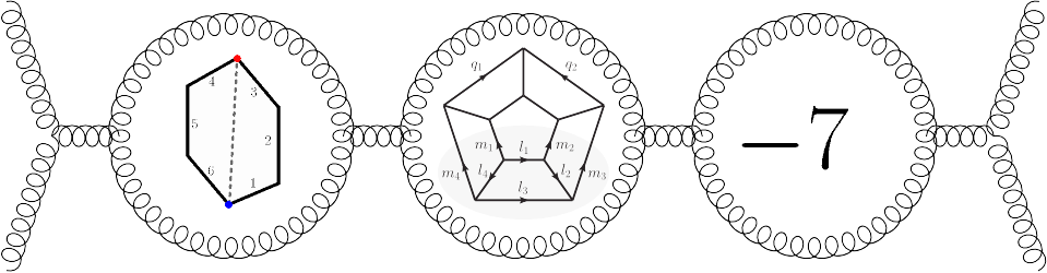
Loops measure precision. They’re called loops because more complicated Feynman diagrams contain “loops” of particles, while the simplest, with no loops at all, are called “trees”. The more loops you include, the more precise your calculation becomes, but it also becomes more complicated.

Legs are the number of particles involved. If two particles collide and bounce off each other, then there are a total of four legs: two from the incoming particles, two from the outgoing ones. Calculations with more legs are almost always more complicated than calculations with fewer.

Most of the time, our end-goal is to calculate things that are relevant to the real world. Usually, this means QCD, or Quantum Chromodynamics, the theory of quarks and gluons. QCD is very complicated, though. Often, we work to hone our techniques on simpler theories first. N=4 super Yang-Mills has been called the simplest quantum field theory, particularly the further simplified, planar version. If you want a basic overview of it, check out the Handy Handbooks tab at the top of my blog. Often, progress in amplitudeology involves adapting tricks from planar N=4 super Yang-Mills to more complicated, and more realistic, theories.

I should point out that our goal in amplitudeology isn’t always to do more complicated calculations. Sometimes, it’s about doing a calculation we already know how to do, but in a way that’s more insightful. This lets us learn more about the theories we’re studying, as well as gaining insights about larger problems like the nature of space and time.

So what sorts of tricks do we use to do all this? Well, there are a few broad categories…

Generalized Unitarity

The prizewinning idea that started it all, generalized unitarity came out of the collaboration of Zvi Bern, Lance Dixon, and David Kosower, starting in the 90’s. The core of the idea is difficult to describe in a quick sentence, but it essentially boils down to noticing that, rather than thinking about every single multi-loop Feynman diagram independently, you can think of loop diagrams as what you get when you sew trees together.

This is a very powerful idea. These days, pretty much everyone who studies amplitudeology learns it, and it’s proven pivotal for a wide array of applications.

In planar N=4 super Yang-Mills it’s one of the techniques that can go to exceptionally high loop order, to six or seven loops. If you drop the “planar” condition, it’s still quite powerful. If you do things right, as Zvi Bern, John Joseph Carrasco, and Henrik Johansson found, you can get results in N=8 supergravity “for free”. This raises what has ended up being one of the big questions of our sub-field: does N=8 supergravity behave like most attempts at theories of quantum gravity, with pesky infinite results that we don’t know how to deal with, or does it behave like N=4 super Yang-Mills, which has no pesky infinities at all? Answering this question requires a dizzying seven-loop calculation, the mystique of which got me in to the field in the first place. Unfortunately, despite diligent efforts from Bern and collaborators, they’ve been stuck at four loops for quite some time. In the meantime they’ve been extending things in all the other amplitudes-directions: more legs, more complicated theories (in this case, supergravity with less supersymmetry), and more insight. Recently, it looks like they may have found a way around this hurdle, so the mystery at seven loops may not be so far away after all.

Generalized Unitarity is also one of the most powerful amplitudes tricks for real-world theories, in particular QCD. In this case, it’s main virtue is in legs, not loops, going up to seven-particles at one loop for practical, LHC-relevant calculations. There’s also a major effort to push this to two loops, with some success.

BCFW Recursion

If generalized unitarity was the trick that got experimentalists to sit up and take notice, BCFW is the one that got the attention of the pure theorists. In the mid-2000s Ruth Britto, Freddy Cachazo, and Bo Feng (later joined by theoretical physics superstar Ed Witten) figured out a way to build up tree amplitudes to any number of legs recursively for any theory, starting with three particles and working their way up. Their method was both fairly efficient and extremely insightful, and it’s another trick that’s made its way into every amplitudeologist’s arsenal. Further developments led to a recursive procedure that could work up to any number of loops in planar N=4 super Yang-Mills, which while not especially efficient did lead to…

The Positive Grassmannian, and the Amplituhedron

The work of Nima Arkani-Hamed, Jacob Bourjaily, Freddy Cachazo, Alexander Goncharov, Alexander Postnikov, and Jaroslav Trnka on the Positive Grassmannian (and more recently the Amplituhedron) has pushed the “more insight” direction impressively far. The Amplituhedron in particular captured the public’s imagination, as well as that of mathematicians, by packaging the all-loop amplitude into a particularly clean, mathematically meaningful form. Now they’re working on pushing this deep understanding to non-planar N=4 super Yang-Mills.

Integration Tricks

Generalized unitarity and the Amplituhedron have one thing in common: neither gives the full result. Calculating scattering amplitudes traditionally is a two-step process: first, add up all possible Feynman diagrams, then add up (integrate) all possible momenta. Generalized unitarity and the Amplituhedron let you skip the diagrams, but in both cases you still need to integrate. There’s a whole lore of integration techniques, from breaking things up into a basis of known “master” integrals (an example paper on this theme here), to attacking the integrations numerically via a process known as sector decomposition (one of the better programs that does this here). Higher-loop integrations are typically quite tough, even with these techniques.

Polylogarithms

These integrals will usually result in a type of mathematical functions called polylogarithms, or transcendental functions. Understanding these functions has led to an enormous amount of progress (and I’m not just saying that because it’s what I work on 😉 ).

It all started when Alexander Goncharov, Mark Spradlin, Cristian Vergu, and Anastasia Volovich figured out how to write a laboriously calculated seventeen-page two-loop six-particle amplitude in just two lines. To do this, they used mathematical properties of polylogarithms that were previously largely unknown to physicists. Their success inspired Lance Dixon, James Drummond, and Johannes Henn to use these methods to guess the correct answer at three loops, work that was completed with my involvement.

Since then, both groups have made a lot of progress. In general, Spradlin, Volovich, and collaborators have been pushing things farther in terms of legs and insight, while Dixon and collaborators have made progress at higher loops. So far we’ve gotten to four loops (here, plus unpublished work), while the others have proposals for any number of particles at two loops and substantial progress for seven particles at three loops.

All of this is still for planar N=4 super Yang-Mills. Using these tricks for more complicated theories is trickier. However, while you usually can’t just guess the answer like you can for N=4, a good understanding of the properties of polylogarithms can still take you quite far.

Integrability

Why did the polylogarithm folks start with six particles? Wouldn’t four or five have been easier?

As it turns out, four and five particle amplitudes are indeed easier, so much so that for planar N=4 super Yang-Mills they’re known up to any loop order. And while a number of elements went in to that result, one that really filled in the details was integrability.

Integrability is tough to describe in a short sentence, but essentially it involves describing highly symmetric systems all in one go, without having to use the step-by-step approximations of perturbation theory. For our purposes, this means bypassing the loop-by-loop perspective altogether.

Integrability is a substantial field in its own right, probably bigger than amplitudeology. There’s a lot going on, and only some of it touches on amplitudes-related topics. When it does, though, it’s quite impressive, with the flagship example being the work of Benjamin Basso, Amit Sever, and Pedro Vieira. They are able to compute amplitudes in planar N=4 super Yang-Mills for any and all loops, instead making an approximation based on the particle momenta. These days, they’re working on making their method more complete and robust, while building up understanding of other structures that might eventually allow them to say something about the non-planar case.

CHY and the Ambitwistor String

Ed Witten’s involvement in BCFW didn’t come completely out of left field. He had shown interest in N=4 super Yang-Mills earlier, with the invention of the twistor string. The twistor string calculates tree amplitudes in N=4 super Yang-Mills as the result of a string-theory-like framework. The advantage to such a framework is that, while normal quantum field theory involves large numbers of different diagrams, string theory only has one diagram “shape” for each loop.

This advantage has been thrust back into the spotlight recently via the work of Freddy Cachazo, Song He, and Ellis Ye Yuan. Their CHY formula works not just for N=4 super Yang-Mills, but for a wide (and growing) variety of other theories, allowing them to examine those theories’ properties in a particularly powerful way. Meanwhile, Lionel Mason and David Skinner have given the CHY formula a more solid theoretical grounding in the form of their ambitwistor string, which they have recently been able to generalize to a loop-level proposal.

Amplitudeology is a large and growing field, and there are definitely important people I haven’t mentioned. Some, like Henriette Elvang and Yu-tin Huang, have been involved with many different things over the years, so there wasn’t a clear place to put them. Others are part of the European community, where there’s a lot of work on string theory amplitudes and on pushing the boundaries of polylogarithms. Still others were left out simply because I ran out of room. I’ve only covered a small part of the field here, but I hope that small part gives you an idea of the richness of the whole.

Hexagon Functions II: Lost in (super)Space

My new paper went up last night.

It’s on a very similar topic to my last paper, actually. That paper dealt with a specific process involving six particles in my favorite theory, N=4 super Yang-Mills. Two particles collide, and after the metaphorical dust settles four particles emerge. That means six “total” particles, if you add the two in with the four out, for a “hexagon” of variables. To understand situations like that, my collaborators and I created “hexagon functions”, formulas that depended on the states of the six particles.

One thing I didn’t emphasize then was that that calculation only applied to one specific choice of particles, one in which all of the particles are Yang-Mills bosons, particles (like photons) created by the fundamental forces. There are lots of other particles in N=4 super Yang-Mills, though. What happens when they collide?

That question is answered by my new paper. Though it may sound surprising, all of the other particles can be taken into account with a single formula. In order to explain why, I have to tell you about something called superspace.

A while back I complained about a blog post by George Musser about the (2,0) theory. One of the things that irked me about that post was his attempt to explain superspace:

Supersymmetry is the idea that spacetime, in addition to its usual dimensions of space and time, has an entirely different type of dimension—a quantum dimension, whose coordinates are not ordinary real numbers but a whole new class of number that can be thought of as the square roots of zero.

This is actually a great way to think about superspace…if you’re already a physicist. If you’re not, it’s not very informative. Here’s a better way to think about it:

As I’ve talked about before, supersymmetry is a relationship between different types of particles. Two particles related by supersymmetry have the same mass, and the same charge. While they can be very different in other ways (specifically, having different spin), supersymmetric particles are described by many of the same equations as each-other. Rather than writing out those equations multiple times, it’s often nicer to write them all in a unified way, and that’s where superspace comes in.

At its simplest, superspace is just a trick used to write equations in a simpler way. Instead of writing down a different equation for each particle we write one equation with an extra variable, representing a “dimension” of supersymmetry. Traveling in that dimension takes you from particle to particle, in the same way that “turning” the theory (as I phrase it here) does, but it does it within the space of a single equation.

That, essentially, is the trick that we use. With four “superspace dimensions”, we can include the four supersymmetries of N=4 super Yang-Mills, showing how the formulas vary when you go beyond the equation from our first paper.

So far, you may be wondering why I’m calling superspace a “dimension”, when it probably sounds like more of a label. I’ve mentioned before that, just because something is a variable, doesn’t mean it counts as a real dimension.

The key difference is that superspace dimensions are related to regular dimensions in a precise way. In a sense, they’re the square roots of regular dimensions. (Though independently, as George Musser described, they’re the square roots of zero: go in the same direction twice in supersymmetry, and you get back where you’re started, going zero distance.) The coexistence of these two seemingly contradictory statements isn’t some sort of quantum mystery, it’s just a consequence of the fact that, mathematically, I’m saying two very different things. I just can’t think of a way to explain them differently without math.

Superspace isn’t a real place…but it can often be useful to think of it that way. In theories with supersymmetry, it can unify the world, putting disparate particles together into a single equation.

Numerics, or, Why can’t you just tell the computer to do it?

When most people think of math, they think of the math they did in school: repeated arithmetic until your brain goes numb, followed by basic algebra and trig. You weren’t allowed to use calculators on most tests for the simple reason that almost everything you did could be done by a calculator in a fraction of the time.

Real math isn’t like that. Mathematicians handle proofs and abstract concepts, definitions and constructions and functions and generally not a single actual number in sight. That much, at least, shouldn’t be surprising.

What might be surprising is that even tasks which seem very much like things computers could do easily take a fair bit of human ingenuity.

In physics, I do a lot of integrals. For those of you unfamiliar with calculus, integrals can be thought of as the area between a curve and the x-axis.

Areas seem like the sort of thing it would be easy for a computer to find. Chop the space into little rectangles, add up all the rectangles under the curve, and if your rectangles are small enough you should get the right answer. Broadly, this is the method of numerical integration. Since computers can do billions of calculations per second, you can chop things up into billions of rectangles and get as close as you’d like, right?

Heck, ten is a lot. Can we just do ten?

Heck, ten is a lot. Can we just do ten?

For some curves, this works fine. For others, though…

Ten might not be enough for this one.

Ten might not be enough for this one.

See how the left side of that plot goes off the chart? That curve goes to infinity. No matter how many rectangles you put on that side, you still won’t have any that are infinitely tall, so you’ll still miss that part of the curve.

Surprisingly enough, the area under this curve isn’t infinite. Do the integral correctly, and you get a result of 2. Set a computer to calculate this integral via the sort of naïve numerical integration discussed above though, and you’ll never find that answer. You need smarter methods: smart humans doing the math, or smart humans programming the computer.

Another way this can come up is if you’re adding up two parts of something that go to infinity in opposite directions. Try to integrate each part by itself and you’ll be stuck.

firstplot

secondplot

But add them together, and you get something quite a bit more tractable.

Yeah, definitely a ten-rectangle job.

Yeah, definitely a ten-rectangle job.

Numerical integration, and computers in general, are a very important tool in a scientist’s arsenal. But in order to use them, we have to be smart, and know what we’re doing. Knowing how to use our tools right can take almost as much expertise and care as working without tools.

So no, I can’t just tell the computer to do it.