Tag Archives: theoretical physics

Update on the Amplituhedron

Awhile back I wrote a post on the Amplituhedron, a type of mathematical object  found by Nima Arkani-Hamed and Jaroslav Trnka that can be used to do calculations of scattering amplitudes in planar N=4 super Yang-Mills theory. (Scattering amplitudes are formulas used to calculate probabilities in particle physics, from the probability that an unstable particle will decay to the probability that a new particle could be produced by a collider.) Since then, they published two papers on the topic, the most recent of which came out the day before New Year’s Eve. These papers laid out the amplituhedron concept in some detail, and answered a few lingering questions. The latest paper focused on one particular formula, the probability that two particles bounce off each other. In discussing this case, the paper serves two purposes:

1. Demonstrating that Arkani-Hamed and Trnka did their homework.

2. Showing some advantages of the amplituhedron setup.

Let’s talk about them one at a time.

Doing their homework

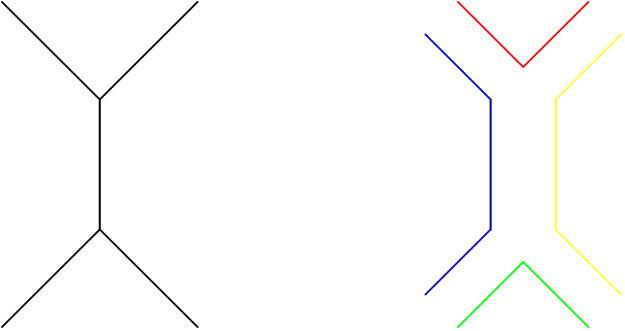
There’s already a lot known about N=4 super Yang-Mills theory. In order to propose a new framework like the amplituhedron, Arkani-Hamed and Trnka need to show that the new framework can reproduce the old knowledge. Most of the paper is dedicated to doing just that. In several sections Arkani-Hamed and Trnka show that the amplituhedron reproduces known properties of the amplitude, like the behavior of its logarithm, its collinear limit (the situation when two momenta in the calculation become parallel), and, of course, unitarity.

What, you heard the amplituhedron “removes” unitarity? How did unitarity get back in here?

This is something that has confused several commenters, both here and on Ars Technica, so it bears some explanation.

Unitarity is the principle that enforces the laws of probability. In its simplest form, unitarity requires that all probabilities for all possible events add up to one. If this seems like a pretty basic and essential principle, it is! However, it and locality (the idea that there is no true “action at a distance”, that particles must meet to interact) can be problematic, causing paradoxes for some approaches to quantum gravity. Paradoxes like these inspired Arkani-Hamed to look for ways to calculate scattering amplitudes that don’t rely on locality and unitarity, and with the amplituhedron he succeeded.

However, just because the amplituhedron doesn’t rely on unitarity and locality, doesn’t mean it violates them. The amplituhedron, for all its novelty, still calculates quantities in N=4 super Yang-Mills. N=4 super Yang-Mills is well understood, it’s well-behaved and cuddly, and it obeys locality and unitarity.

This is why the amplituhedron is not nearly as exciting as a non-physicist might think. The amplituhedron, unlike most older methods, isn’t based on unitarity and locality. However, the final product still has to obey unitarity and locality, because it’s the same final product that others calculate through other means. So it’s not as if we’ve completely given up on basic principles of physics.

Not relying on unitarity and locality is valuable. For those who research scattering amplitudes, it has often been useful to try to “eliminate” one principle or another from our calculations. 20 years ago, avoiding Feynman diagrams was the key to finding dramatic simplifications. Now, many different approaches try to sidestep different principles. (For example, while the amplituhedron calculates an integrand and leaves a final integral to be done, I’m working on approaches that never employ an integrand.)

If we can avoid relying on some “basic” principle, that’s usually good evidence that the principle might be a consequence of something even more basic. By showing how unitarity can arise from the amplituhedron, Arkani-Hamed and Trnka have shown that a seemingly basic principle can come out of a theory that doesn’t impose it.

Advantages of the Amplituhedron

Not all of the paper compares to old results and principles, though. A few sections instead investigate novel territory, and in doing so show some of the advantages and disadvantages of the amplituhedron.

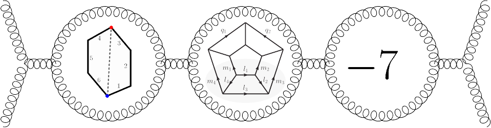
Last time I wrote on this topic, I was unclear on whether the amplituhedron was more efficient than existing methods. At this point, it appears that it is not. While the formula that the amplituhedron computes has been found by other methods up to seven loops, the amplituhedron itself can only get up to three loops or so in practical cases. (Loops are a way that calculations are classified in particle physics. More loops means a more complex calculation, and a more precise final result.)

The amplituhedron’s primary advantage is not in efficiency, but rather in the fact that its mathematical setup makes it straightforward to derive interesting properties for any number of loops desired. As Trnka occasionally puts it, the central accomplishment of the amplituhedron is to find “the question to which the amplitude is the answer”. By being able to phrase this “question” mathematically, one can be very general, which allows them to discover several properties that should hold no matter how complex the rest of the calculation becomes. It also has another implication: if this mathematical question has a complete mathematical answer, that answer could calculate the amplitude for any number of loops. So while the amplituhedron is not more efficient than other methods now, it has the potential to be dramatically more efficient if it can be fully understood.

All that said, it’s important to remember that the amplituhedron is still limited in scope. Currently, it applies to a particular theory, one that doesn’t (and isn’t meant to) describe the real world. It’s still too early to tell whether similar concepts can be defined for more realistic theories. If they can, though, it won’t depend on supersymmetry or string theory. One of the most powerful techniques for making predictions for the Large Hadron Collider, the technique of generalized unitarity, was first applied to N=4 super Yang-Mills. While the amplituhedron is limited now, I would not be surprised if it (and its competitors) give rise to practical techniques ten or twenty years down the line. It’s happened before, after all.

Elegance, Not So Mysterious

You’ll often hear theoretical physicists in the media referring to one theory or another as “elegant”. String theory in particular seems to get this moniker fairly frequently.

It may often seem like mathematical elegance is some sort of mysterious sixth sense theorists possess, as inexplicable to the average person as color to a blind person. What’s “elegant” about string theory, after all?

Before explaining elegance, I should take a bit of time to say what it’s not. Elegance isn’t Occam’s razor. It isn’t naturalness, either. Both of those concepts have their own technical definitions.

Elegance, by contrast, is a much hazier, and yet much simpler, notion. It’s hazy enough that any definition could provoke arguments, but I can at least give you an approximate idea by telling you that an elegant theory is simple to describe, if you know the right terms. Often, it is simpler than the phenomenon that it explains.

How does this apply to something like string theory? String theory seems to be incredibly complicated: ten dimensions, curled up in a truly vast number of different ways, giving rise to whole spectrums of particles.

That said, the basic idea is quite simple. String theory asks the question: what if, in addition to fundamental point-particles (zero dimensional objects), there were fundamental objects of other dimensions? That idea leads to complicated consequences: if your theory is going to produce all the particles of the real world then you need the ten dimensions and the supersymmetry and yadda yadda. But the basic idea is simple to describe. An elegant theory can have very complicated consequences, but still be simple to describe.

This, broadly, is the sort of explanation theoretical physicists look for. Math is the kind of field where the same basic systems can describe very complex phenomena. Since theoretical physics is about describing the world in terms of math, the right explanation is usually the most elegant.

This can occasionally trip physicists up when they migrate to other careers. In biology, for example, the elegant solution is often not the right one, because evolution doesn’t care about elegance: evolution just grabs whatever is within reach. Financial systems and economics occasionally have similar problems. All this is to say that while elegance is an important thing for a physicist to strive for, sometimes we have to be careful about it.

Blackboards, Again

Recently I had the opportunity to give a blackboard talk. I’ve talked before about the value of blackboards, how they facilitate collaboration and can even be used to get work done. What I didn’t feel the need to explain was their advantages when giving a talk.

No, the blackboard behind me isn't my talk.

No, the blackboard behind me isn’t my talk.

When I mentioned I was giving a blackboard talk, some of my friends in other fields were incredulous.

“Why aren’t you using PowerPoint? Do you people hate technology?”

So why do theorists (and mathematicians) do blackboard talks, when many other fields don’t?

Typically, a chemist can’t bring chemicals to a talk. A biologist can’t bring a tank of fruit flies or zebrafish, and a psychologist probably shouldn’t bring in a passel of college student test subjects. As a theorist though, our test subjects are equations, and we can absolutely bring them into the room.

In the most ideal case, a talk by a theorist walks you through their calculation, reproducing it on the blackboard in enough detail that you can not only follow along, but potentially do the calculation yourself. While it’s possible to set up a calculation step by step in PowerPoint, you don’t have the same flexibility to erase and add to your equations, which becomes especially important if you need to clarify a point in response to a question.

Blackboards also often give you more space than a single slide. While your audience still only pays attention to a slide-sized area of the board at one time, you can put equations up in one area, move away, and then come back to them later. If you leave important equations up, people can remind themselves of them on their own time, without having to hold everybody up while you scroll back through the slides to the one they want to see.

Using a blackboard well is a fine art, and one I’m only beginning to learn. You have to know what to erase and what to leave up, when to pause to allow time to write or ask questions, and what to say while you’re erasing the board. You need to use all the quirks of the medium to your advantage, to show people not just what you did, but how and why you did it.

That’s why we use blackboards. And if you ask why we can’t do the same things with whiteboards, it’s because whiteboards are terrible. Everybody knows that.

What are Vacua? (A Point about the String Landscape)

A couple weeks back, there was a bit of a scuffle between Matt Strassler and Peter Woit on the subject of predictions in string theory (or more properly, the question of whether any predictions can be made at all). As a result, Strassler has begun a series on the subject of quantum field theory, string theory, and predictions.

Strassler hasn’t gotten to the topic of string vacua yet, but he’s probably going to cover the subject in a future post. While his take on the subject is likely to be more expansive and precise than mine, I think my perspective on the problem might still be of interest.

Let’s start with the basics: one of the problems often cited with string theory is the landscape problem, the idea that string theory has a metaphorical landscape of around 10^500 vacua.

What are vacua?

Vacua is the plural of vacuum.

Ok, and?

A vacuum is empty space.

That’s what you thought, right? That’s the normal meaning of vacuum. But if a vacuum is empty, how can there be more than one of them, let alone 10^500?

“Empty” is subjective.

Now we’re getting somewhere. The problem with defining a concept like “empty space” in string theory or field theory is that it’s unclear what precisely it should be empty of. Naively, such a space should be empty of “stuff”, or “matter”, but our naive notions of “matter” don’t apply to field theory or string theory. In fact, there is plenty of “stuff” that can be present in “empty” space.

Think about two pieces of construction paper. One is white, the other is yellow. Which is empty? Neither has anything drawn on it, so while one has a color and the other does not, both are empty.

“Empty space” doesn’t come in multiple colors like construction paper, but there are equivalent parameters that can vary. In quantum field theory, one option is for scalar fields to take different values. In string theory, different dimensions can be curled up in different ways (as an aside, when string theory leads to a quantum field theory often these different curling-up shapes correspond to different values for scalar fields, so the two ideas are related).

So if space can have “stuff” in it and still count as empty, are there any limits on what can be in it?

As it turns out, there is a quite straightforward limit. But to explain it, I need to talk a bit about why physicists care about vacua in the first place.

Why do physicists care about vacua?

In physics, there is a standard modus operandi for solving problems. If you’ve taken even a high school physics course, you’ve probably encountered it in some form. It’s not the only way to solve problems, but it’s one of the easiest. The idea, broadly, is the following:

First get the initial conditions, and then use the laws of physics to see what happens next.

In high school physics, this is how almost every problem works: your teacher tells you what the situation is, and you use what you know to figure out what happens next.

In quantum field theory, things are a bit more subtle, but there is a strong resemblance. You start with a default state, and then find the perturbations, or small changes, around that state.

In high school, your teacher told you what the initial conditions were. In quantum field theory, you need another source for the “default state”. Sometimes, you get that from observations of the real world. Sometimes, though, you want to make a prediction that goes beyond what your observations tell you. In that case, one trick often proves useful:

To find the default state, find which state is stable.

If your system starts out in a state that is unstable, it will change. It will keep changing until eventually it changes into a stable state, where it will stop changing. So if you’re looking for a default state, that state should be one in which the system is stable, where it won’t change.

(I’m oversimplifying things a bit here to make them easier to understand. In particular, I’m making it sound like these things change over time, which is a bit of a tricky subject when talking about different “default” states for the whole of space and time. There’s also a cool story connected to this about why tachyons don’t exist, which I’d love to go into for another post.)

Since we know that the “default” state has to be stable, if there is only one stable state, we’ve found the default!

Because of this, we can lay down a somewhat better definition:

A vacuum is a stable state.

There’s more to the definition than this, but this should be enough to give you the feel for what’s going on. If we want to know the “default” state of the world, the state which everything else is just a small perturbation on top of, we need to find a vacuum. If there is only one plausible vacuum, then our work is done.

When there are many plausible vacua, though, we have a problem. When there are 10^500 vacua, we have a huge problem.

That, in essence, is why many people despair of string theory ever making any testable predictions. String theory has around 10^500 plausible vacua (for a given, technical, meaning of plausible).

It’s important to remember a few things here.

First, the reason we care about vacuum states is because we want a “default” to make predictions around. That is, in a sense, a technical problem, in that it is an artifact of our method. It’s a result of the fact that we are choosing a default state and perturbing around it, rather than proving things that don’t depend on our choice of default state. That said, this isn’t as useful an insight as it might appear, and as it turns out there is generally very little that can be predicted without choosing a vacuum.

Second, the reason that the large number of vacua is a problem is that if there was only one vacuum, we would know which state was the default state for our world. Instead, we need some other method to pick, out of the many possible vacua, which one to use to make predictions. That is, in a sense, a philosophical problem, in that it asks what seems ostensibly to be a philosophical question: what is the basic, default state of the universe?

This happens to be a slightly more useful insight than the first one, and it leads to a number of different approaches. The most intuitive solution is to just shrug and say that we will see which vacuum we’re in by observing the world around us. That’s a little glib, since many different vacua could lead to very similar observations. A better tactic might be to try to make predictions on general grounds by trying to see what the world we can already observe implies about which vacua are possible, but this is also quite controversial. And there are some people who try another approach, attempting to pick a vacuum not based on observations, but rather on statistics, choosing a vacuum that appears to be “typical” in some sense, or that satisfies anthropic constraints. All of these, again, are controversial, and I make no commentary here about which approaches are viable and which aren’t. It’s a complicated situation and there are a fair number of people working on it. Perhaps, in the end, string theory will be ruled un-testable. Perhaps the relevant solution is right under peoples’ noses. We just don’t know.

Brown, Blue, and Birds

I gave a talk at Brown this week, so this post may be shorter than usual. On the topic of Brown I don’t have much original to say: the people were friendly, the buildings were brownish-colored, and bringing a car there was definitely a bad idea. Don’t park at Brown. Not even then.

There’s a quote from Werner Heisenberg that has been making the rounds of the internet. It comes out of a 1976 article by Felix Bloch where he describes taking a walk with Heisenberg, when the discussion turned to the subject of space and time:

I had just read Weyl’s book Space, Time and Matter, and under its influence was proud to declare that space was simply the field of linear operations.

“Nonsense,” said Heisenberg, “space is blue and birds fly through it.”

Heisenberg’s point is that sometimes in physics you need to ask what your abstractions are really describing. You need to make sure that you haven’t stretched your definitions too badly away from their original inspiration.

When people first hear that string theory requires eleven dimensions, many wonder if this point applies. In mathematics, it’s well known that a problem can be described in many dimensions more than the physical dimensions of space. There’s a lovely example in the book Flatterland (a sequel to Flatland, a book which any math-y person should read at least once) of the dimensions of a bike. The bike’s motion through space gives three dimensions: up/down, backward/forward, and left/right. However, the bike can move in other ways: its gears can each be in a different position, as can its handlebars, as can the wheels…in the end, a bike can be envisioned as having many more “dimensions” than our normal three-dimensional space, each corresponding to some internal position.

Is string theory like this? No.

The first hint of the answer comes from something called F theory. String theory is part of something larger called M theory, and since M theory has eleven dimensions this is usually the number of dimensions given. But F theory contains string theory in a certain sense as well, only F theory contains twelve dimensions.

So why don’t string theorists say that the world has twelve dimensions?

As it turns out, the extra dimension added by F theory isn’t “really” a dimension. It’s much more like the mathematical dimensions of a bike’s gears and wheels than it is like the other eleven dimensions of M theory.

What’s the difference? What, according to a string theorist, is the definition of a dimension of space?

It’s simple: Space is “blue” (or colorless, I suppose). Birds (and particles, and strings, and membranes) fly in it.

We’re using the same age-old distinction that Heisenberg was, in a way. What is space? Space is just a place where things can move, in the same way they move in our usual three dimensions. Space is where you have momentum, where that momentum can change your position. Space is where forces act, the set of directions in which something can be pulled or pushed in a symmetric way. Space can’t be reduced, at least not without a lot of tricks: a bird flying isn’t just another description of a lizard crawling, not in the way a bicycle’s gears moving can be thought of as turning through our normal three dimensions without any extra ones. And while F theory doesn’t fit this criterion, M theory really does. The membranes of M theory fly around in eleven dimensional space-time, just like a bird moves through three space and one time dimensions.

Space for a string theorist isn’t any crazier or more abstract than it is for you. It’s just a place where things can move.

Planar vs. Non-Planar: A Colorful Story

Last week, I used two terms, planar theory and non-planar theory, without defining them. This week, I’m going to explain what they mean, and why they’re important.

Suppose you’re working with a Yang-Mills theory (not necessarily N=4 super Yang-Mills. To show you the difference between planar and non-planar, I’ll draw some two-loop Feynman diagrams for a process where two particles go in and two particles come out:

planarity1

The diagram on your left is planar, while the diagram on your right is non-planar. The diagram on the left can be written entirely on a flat page (or screen), with no tricks. By contrast, with the diagram on the right I have to cheat and make one of the particle lines jump over another one (that’s what the arrow is meant to show). Try as you might, you can’t twist that diagram so that it lies flat on a plane (at least not while keeping the same particles going in and out). That’s the difference between planar and non-planar.

Now, what does it mean for a theory to be planar or non-planar?

Let’s review some facts about Yang-Mills theories. (For a more detailed explanation, see here). In Yang-Mills there are a certain number of colors, where each one works a bit like a different kind of electric charge. The strong force, the force that holds protons and neutrons together, has three colors, usually referred to as red, blue, and green (this is of course just jargon, not the literal color of the particles).

Forces give rise to particles. In the case of the strong force, those particles are called gluons. Each gluon has a color and an anti-color, where you can think of the color like a positive charge and the anti-color like a negative charge. A given gluon might be red-antiblue, or green-antired, or even red-antired.

While the strong force has three colors, for this article it will be convenient to pretend that there are four: red, green, blue, and yellow.

An important principle of Yang-Mills theories is that color must be conserved. Since anti-colors are like negative colors, they can cancel normal colors out. So if you’ve got a red-antiblue gluon that collides with a blue-antigreen gluon, the blue and antiblue can cancel each other out, and you can end up with, for example, red-antiyellow and yellow-antigreen instead.

Let’s consider that process in particular. There are lots of Feynman diagrams you can draw for it, let’s draw one of the simplest ones first:

planarity2

The diagram on the left just shows the process in terms of the particles involved: two gluons go in, two come out.

The other diagram takes into account conservation of colors. The red from the red-antiblue gluon becomes the red in the red-antiyellow gluon on the other side. The antiblue instead goes down and meets the blue from the blue-antigreen gluon, and both vanish in the middle, cancelling each other out. It’s as if the blue color entered the diagram, then turned around backwards and left it again. (If you’ve ever heard someone make the crazy-sounding claim that antimatter is normal matter going backwards in time, this is roughly what they mean.)

From this diagram, we can start observing a general principle: to make sure that color is conserved, each line must have only one color.

Now let’s try to apply this principle to the two-loop diagrams from the beginning of the article. If you draw double lines like we did in the last example, fill in the colors, and work things out, this is what you get:

planarity3

What’s going on here?

In the diagram on the left, you see the same lines as the earlier diagram on the outside. On the inside, though, I’ve drawn two loops of color, purple and pink.

I drew the lines that way because, just based on the external lines, you don’t know what color they should be. They could be red, or yellow, or green, or blue. Nothing tells you which one is right, so all of them are possible.

Remember that for Feynman diagrams, we need to add up every diagram we can draw to get the final result. That means that there are actually four times four or sixteen copies of this diagram, each one with different colors in the loops.

Now let’s look at the other diagram. Like the first one, it’s a diagram with two loops. However, in this case, the inside of both loops is blue. If you like, you can try to trace out the lines in the loops. You’ll find that they’re all connected together. Because this diagram is non-planar, color conservation fixes the color in the loops.

So while there are sixteen copies of the first diagram, there is only one possible version of the second one. Since you add all the diagrams together, that means that the first diagram is sixteen times more important than the second diagram.

Now suppose we had more than four colors. Lots more.

More than that…

With ten colors, the planar diagrams are a hundred times more important. With a hundred colors, they are ten thousand times more important. Keep increasing the number of colors, and it gets to the point where you can honestly say that the non-planar diagrams don’t matter at all.

What, then, is a “planar theory”?

A planar theory is a theory with a very large (infinite) number of colors.

In a planar theory, you can ignore the non-planar diagrams and focus only on the planar ones.

Nima Arkani-Hamed’s Amplituhedron method applies to the planar version of N=4 super Yang-Mills. There is a lot of progress on the planar version of the theory, and it is because the restriction to planar diagrams makes things simpler.

However, sometimes you need to go beyond planar diagrams. There are relationships between planar and non-planar diagrams, based on the ways that you can pair different colors together in the theory. Fully understanding this relationship is powerful for understanding Yang-Mills theory, but, as it turns out, it’s also the key to relating Yang-Mills theory to gravity! But that’s a story for another post.

The Amplituhedron and Other Excellently Silly Words

Nima Arkani-Hamed recently gave a talk at the Simons Center on the topic of what he and Jaroslav Trnka are calling the Amplituhedron.

There’s an article on it in Quanta Magazine. The article starts out a bit hype-y for my taste (too much language of importance, essentially), but it has several very solid descriptions of the history of the situation. I particularly like how the author concisely describes the Feynman diagram picture in the space of a single paragraph, and I would recommend reading that part even if you don’t have time to read the whole article. In general it’s worth it to get a picture of what’s going on.

That said, I obviously think I can clear a few things up, otherwise I wouldn’t be writing about it, so here I go!

“The” Amplituhedron

Nima’s new construction, the Amplituhedron, encodes amplitudes (building blocks of probabilities in particle physics) in N=4 super Yang-Mills as the “area” of a multi-dimensional analog of a polyhedron (hence, Amplitu-hedron).

Now, I’m a big supporter of silly-sounding words with amplitu- at the beginning (amplitudeologist, anyone?), and this is no exception. Anyway, the word Amplitu-hedron isn’t what’s confusing people. What’s confusing people is the word the.

When the Quanta article says that Nima has found “the” Amplituhedron, it makes it sound like he has discovered one central formula that somehow contains the whole universe. If you read the comments, many readers went away with that impression.

In case you needed me to say it, that’s not what is going on. The problem is in the use of the word “the”.

Suppose it was 1886, and I told you that a fellow named Carl Benz had invented “the Automobile”, a marvelous machine that can get everyone to work on time (as well as become the dominant form of life on Long Island).

My use of “the” might make you imagine that Benz invented some single, giant machine that would roam across the country, picking people up and somehow transporting everyone to work. You’d be skeptical of this, of course, expecting that long queues to use this gigantic, wondrous machine would swiftly ruin any speed advantage it might possess…

The Automobile, here to take you to work.

Or, you could view “the” in another light, as indicating a type of thing.

Much like “the Automobile” is a concept, manifested in many different cars and trucks across the country, “the Amplituhedron” is a concept, manifested in many different amplituhedra, each corresponding to a particular calculation that we might attempt.

Advantages…

Each amplituhedron has to do with an amplitude involving a specific number of particles, with a particular number of internal loops. (The Quanta article has a pretty good explanation of loops, here’s mine if you’d rather read that). Based on the problem you’re trying to solve, there are a set of rules that you use to construct the particular amplituhedron you need. The “area” of this amplituhedron (in quotation marks because I mean the area in an abstract, mathematical sense) is the amplitude for the process, which lets you calculate the probability that whatever particle physics situation you’re describing will happen.

Now, we already have many methods to calculate these probabilities. The amplituhedron’s advantage is that it makes these calculations much simpler. What was once quite a laborious and complicated four-loop calculation, Nima claims can be done by hand using amplituhedra. I didn’t get a chance to ask whether the same efficiency improvement holds true at six loops, but Nima’s description made it sound like it would at least speed things up.

[Edit: Some of my fellow amplitudeologists have reminded me of two things. First, that paper I linked above paved the way to more modern methods for calculating these things, which also let you do the four-loop calculation by hand. (You need only six or so diagrams). Second, even back then the calculation wasn’t exactly “laborious”, there were some pretty slick tricks that sped things up. With that in mind, I’m not sure Nima’s method is faster per se. But it is a fast method that has the other advantages described below.]

The amplituhedron has another, more sociological advantage. By describing the amplitude in terms of a geometrical object rather than in terms of our usual terminology, we phrase things in a way that mathematicians are more likely to understand. By making things more accessible to mathematicians (and the more math-headed physicists), we invite them to help us solve our problems, so that together we can come up with more powerful methods of calculation.

Nima and the Quanta article both make a big deal about how the amplituhedron gets rid of the principles of locality and unitarity, two foundational principles of quantum field theory. I’m a bit more impressed by this than Woit is. The fine distinction that needs to be made here is that the amplituhedron isn’t simply “throwing out” locality and unitarity. Rather, it’s written in such a way that it doesn’t need locality and unitarity to function. In the end, the formulas it computes still obey both principles. Nima’s hope is that, now that we are able to write amplitudes without needing locality and unitarity, if we end up having to throw out either of those principles to make a new theory we will be able to do so. That’s legitimately quite a handy advantage to have, it just doesn’t mean that locality and unitarity must be thrown out right now.

…and Disadvantages

It’s important to remember that this whole story is limited to N=4 super Yang-Mills. Nima doesn’t know how to apply it to other theories, and nobody else seems to have any good ideas either. In addition, this only applies to the planar part of the theory. I’m not going to explain what that term means here; for now just be aware that while there are tricks that let you “square” a calculation in super Yang-Mills to get a similar calculation in quantum gravity, those tricks rely on having non-planar data, or information beyond the planar part of the theory. So at this point, this doesn’t give us any new hints about quantum gravity. It’s conceivable that physicists will find ways around both of these limits, but for now this result, though impressive, is quite limited.

Nima hasn’t found some sort of singular “jewel at the heart of physics”. Rather, he’s found a very slick, very elegant, quite efficient way to make calculations within one particular theory. This is profound, because it expresses things in terms that mathematicians can address, and because it shows that we can write down formulas without relying on what are traditionally some of the most fundamental principles of quantum field theory. Only time will tell whether Nima or others can generalize this picture, taking it beyond planar N=4 super Yang-Mills and into the tougher theories that still await this sort of understanding.

The (2, 0) Theory: What is it, though?

Part Three of a Series on the (2, 0) Theory

If you’ve been following this series, you know that the (2, 0) theory describes what it’s like to live on a five dimensional membrane in M theory. You know it’s got five scalar fields, and four chiral fermions (and hopefully you have a rough idea of what those things are). And if you’ve been reading for longer, you’ve probably heard me mention that a theory is essentially a list of quantum fields. So if I’m going to define the (2, 0) theory for you, I ought to, at the very least, list its quantum fields.

This is where things get tricky, and where unfortunately I will have to get a big vague. Some of the quantum fields in the (2, 0) theory are things I’ve talked about before: the five scalars and the four fermions. The remaining field, though, is different, and it’s the reason why the (2, 0) theory is so mysterious.

I’ll start by throwing around some terminology. Normally, I’d go back and explain it, but in this case there’s simply too much. My aim here is to give the specialists reading this enough to understand what I’m talking about. Then I’ll take a few paragraphs to talk about what the implications of all this jargon are for a general understanding.

The remaining field in the (2, 0) theory is a two-form, or an antisymmetric, two-index tensor, with a self-dual field strength. It comes from the gauge orientation zero modes of the M5-brane. It is not a Yang-Mills field. However, it is non-abelian, that is, it “interacts with itself” in a similar way to how a Yang-Mills field does.

While I can give examples of familiar Yang-Mills fields, fermions, and now with the Higgs even scalars, I can’t give you a similar example of a fundamental two-form field. That’s because in our four dimensional world, such a field doesn’t make sense. It only makes sense in six or more dimensions.

The problem with understanding this isn’t just a matter of not having examples in the real world, though. We can invent a wide variety of unobserved fields, and in general have no problem calculating their hypothetical properties. The problem is that, in the case of the two-form field of the (2, 0) theory, we don’t know how to properly do calculations about it.

There are a couple different ways to frame the issue. One is that, while we know roughly which fields should interact with which other fields, there isn’t a mathematically consistent way to write down how they do so. Any attempt results in a formula with some critical flaw that keeps it from being useful.

The other way to frame the problem is to point out that every Yang-Mills force has a number that determines how powerful it is, called the coupling constant. As I discuss here, it is the small size of the coupling constant that allows us to calculate only the simplest Feynman diagrams and still get somewhat accurate results.

The (2, 0) theory has no coupling constant. There is no parameter that, if it was small, would allow you to only look at some diagrams and not others. In the (2, 0) theory, every diagram is equally important.

When people say that the (2, 0) theory is “irreducibly quantum”, this is what they’re referring to: we can’t separate out the less-quantum (lower loops) bits from the more quantum (higher loops) bits. The theory simply is quantum, inherently and uniformly so.

This is what makes it so hard to understand, what makes it sexy and mysterious and Mara Jade-like. If we could understand it, the payoffs would be substantial: M theory has a similar problem, so a full understanding of the (2, 0) theory might pave the way to a full understanding of M theory, which, unlike the (2, 0) theory, really is supposed to be a theory of everything.

And there is progress…somewhat, anyway. Twisting one of the six dimensions of the (2, 0) theory around in a circle gives you N=4 super Yang-Mills in five dimensions, while another circle brings it down to four dimensions. Because super Yang-Mills is so well-understood, this gives us a tantalizing in-road to understanding the (2, 0) theory. I’ve worked a bit on this myself.

Perhaps a good way to summarize the situation would be to say that, while N=4 super Yang-Mills is interesting because of how much we know about it, the (2, 0) theory is interesting because, contrary to expectations, we can do something with it at all. Every time someone comes up with a novel method for understanding quantum field theories, you can rest assured that they will end up trying to apply it to the (2, 0) theory. One of them might even work.

The (2, 0) Theory: What does it mean?

Part Two of a Series on the (2, 0) Theory

Apologies in advance. This is going to be a long one.

So now that you know that the (2, 0) theory is the world-volume theory of an M5-brane, you might be asking what the hell (2, 0) means. Why is this theory labeled with an arcane bunch of numbers rather than words like any sensible theory?

To explain that, we have to talk a bit about how we count supersymmetries. As I talked about with N=4 super Yang-Mills, supersymmetry is a relationship between particles of different spins, and since one particle can be related in this way to more than one other particle, we indicated the number of different related particles by the number N. (I’d recommend reading those posts to understand this one. If you need a quick summary, spin is a way of categorizing particles, with spin 1 corresponding to forces of nature like electromagnetism and the Yang-Mills forces in general, while spin ½ corresponds to the types of particles that make up much of everyday matter, like electrons and quarks.)

As it turns out, we count the number of supersymmetries N differently in different dimensions. The reasons are fairly technical, and are related to the fact that spin ½ particles are more complicated in higher dimensions. The end result is that while super Yang-Mills has N=4 in four dimensions (three space one time), in six dimensions it only has N=2 (in case you’re curious, it goes all the way down to N=1 in ten dimensions).

The “2” in the (2, 0) theory means the same thing as that N=2. However, the (2, 0) theory is very different from super Yang-Mills, and that’s where the other number in the pair comes in. To explain this, I have to talk a bit about something called chirality.

Chirality is a word for handedness. If you’re given a right-handed glove, no matter what you do you can’t rotate it to turn it into a left-handed glove. The only way you could change a right-handed glove into a left-handed glove would be to flip it through a mirror, like Alice through the looking glass.

Particles often behave similarly. While they don’t have fingers to flip, they do have spin.

I told you earlier to think of spin as just a way to classify particles. That’s still the best way for you to think about it, but in order to explain chirality I have to mention that spin isn’t just an arbitrary classification scheme, it’s a number that corresponds to how fast a particle is “spinning”.

Here I have to caution that the particle isn’t necessarily literally spinning. Rather, it acts as if it were spinning, interacting with other objects as if it were spinning with a particular speed. If you’ve ever played with a gyroscope, you know that a spinning object behaves differently from a non-spinning one: the faster it spins, the harder it is to change the direction in which it is spinning.

Suppose that a particle is flying at you head-on. If you measured the particle’s spin, it would appear to be spinning either clockwise or counterclockwise, to the left or to the right. This choice, left or right, is the particle’s chirality.

L for left, R for right, V and p show which way the particle is going.

The weird thing is that there are some particles that only spin one way. For example, every neutrino that has been discovered has left-handed chirality. In general when a fermion only spins one way we call it a chiral fermion.

What does this have to do with the (2, 0) theory?

Supersymmetry relates particles of spin X to particles of spin X-½.  As such, you can look at supersymmetry as taking the original particle, and “subtracting” a particle of spin ½. These aren’t really particles, but they share some properties, and those properties can include chirality. You can have left-supersymmetry, and right-supersymmetry.

So what does (2, 0) mean? It means that not only is the (2, 0) theory an N=2 theory in six dimensions, but those two supersymmetries are chiral. They are only left-handed (or, if you prefer, only right-handed). By contrast, super Yang-Mills in six dimensions is a (1, 1) theory. It has one left-handed supersymmetry, and one right-handed supersymmetry.

We can now learn a bit more about the sorts of particles in the (2, 0) theory.

As I said when discussing N=4 super Yang-Mills, N=4 is the most supersymmetry you can have in Yang-Mills in four dimensions. Any more, and you need to include gravity.  Recall that the (2, 0) theory comes from the behavior of M5-branes in M theory. M theory includes gravity, which means that it can go higher than N=4.

How high? As it turns out, the maximum including gravity (which I will explain a bit more when I do a series on supergravity) is N=8. That’s in four dimensions, however. In M theory’s native eleven dimensions, this is just N=1. In six dimensions, where the (2, 0) theory lives, this becomes N=4. More specifically, including information about chirality, its supersymmetry is (2, 2).

So if M theory in six dimensions has (2, 2) symmetry, how to we get to (2, 0)? What happens to the other ( ,2)?

As I talked about in the last post, the varying position of the M5-brane in the other five dimensions gives rise to five scalar fields. In a way, we have broken the symmetry between the eleven dimensions of M theory, treating five of them differently from the other six.

It turns out that supersymmetry is closely connected to the symmetry of space and time. What this means in practice is that when you break the symmetry of space-time, you can also break supersymmetry, reducing the number N of symmetries. Here, the M5-brane breaks supersymmetry from (2, 2) to (2, 0), so two of the supersymmetries are broken.

Just like the position of the M5-brane can vary, so too can the specific supersymmetries broken. What this means is that just like the numbers for the positions become scalar fields, the choices of supersymmetry to be broken become new fermion fields. Because supersymmetry is broken in a chiral way, these new fermion fields are chiral, which for technical reasons ends up meanings that because of the two broken supersymmetries, there are four new chiral fermions.

So far, we know that the (2, 0) theory has five scalar fields, and four chiral fermions. But scalar fields and chiral fermions are pretty ordinary, surely not as mysterious as the Emperor, or even Mara Jade. What makes the (2, 0) theory so mysterious, so difficult to deal with? What makes it, in a word, sexy? Tune in next week to find out!

The (2, 0) Theory: Where does it come from?

Part One of a Series on the (2, 0) Theory

By semi-popular demand, I’m doing a guide on the (2, 0) theory. Over the course of this guide I’ll try to explain where the (2, 0) theory comes from, what its name means, and, more elusively, what it’s actually about.

The (2, 0) theory doesn’t get much press coverage, and when it does, it’s a bit silly. The article I just linked compares it to Star Wars’ Emperor Palpatine, in analogy with what George Musser and perhaps others call the Darth Vader theory, or N=4 super Yang-Mills.

The metaphor, as far as I can parse it, is the following: while N=4 super Yang-Mills is solid, powerful, and important (like Darth Vader), the (2, 0) theory is mysterious and yet somehow even more central (like the Emperor).

The thing is, while the (2, 0) theory is indeed sexy and mysterious, it isn’t especially central. Laymen haven’t heard of it for good reason: it’s really only specialists in the field who have a reason to be interested in it. So really, it’s more like the Mara Jade theory.

If you don’t know who this is, that’s my point

The (2, 0) theory is very much a theory, in the same sense as N=4 super Yang-Mills. It isn’t a “theory of everything”, and it isn’t supposed to describe the real world. With that in mind, let’s talk about the sort of world it does describe.

There are two ways to “define” the (2, 0) theory. One of them is to take a particular type of string theory (type IIB) with ten dimensions (nine space dimensions and one dimension for time), and twist four of those dimensions into a particular shape (called a K3 surface). There are six dimensions left (five space, one time), and in those six dimensions the world obeys the (2, 0) theory.

That definition may not seem particularly illuminating, and it really isn’t. You can get almost any theory in physics by taking some type of string theory and twisting up some of the dimensions in a particular way, so unless you’re familiar with that particular type of string theory or the particular shape of the dimensions, you don’t learn anything from that definition.

The second definition, though, is more appealing. The (2, 0) theory can be defined as the world-volume theory of a five-dimensional object called an M5-brane.

A world-volume theory is a theory that describes what it is like to live inside of the volume of some object, so that the object is your whole world. To understand what that means, think about Flatland.

Think upward, not northward

In Edwin A. Abbott’s Flatland, the characters are two-dimensional shapes living in a two-dimensional world. Because their whole world is two-dimensional, they cannot imagine a third dimension. Despite that, there is a third dimension, as demonstrated by a sphere who floats through the world one day and upsets the main character’s life. The theory of physics in Flatland, then, is the world-volume theory of a two-dimensional plane in three-dimensional space.

Imagine that the two-dimensional plane of Flatland was flexible, that is, more like a two-dimensional membrane. Such a membrane could move back and forth in the third dimension, rippling up and down.

Now remember that, in Flatland, nobody can imagine a third dimension. So if you are within Flatland, and the world around you is bouncing up and down, can you notice?

The answer is a counter-intuitive yes. It’s easy if there is gravity in the third dimension: when the world curves up, it would get harder to climb up, while if the world curves down, it would be easier. Even if there isn’t gravity, though, you can still notice the changes in energy. It takes energy to set the world vibrating, and that energy has to come from somewhere. That energy can come from movement within your dimension. What a Flatlander would observe, then, would be processes that seem to violate conservation of energy, by losing more energy than they put in: instead, that energy would go to making the world wiggle.

What a Flatland scientist would observe, then, would be a world in which there is some number that can change from place to place, and that can oscillate, carrying energy as it does so. Those of you who remember my older posts might recognize what’s going on here: this is precisely the way in which you discover the existence of a scalar field!

An M5-brane is a five-dimensional membrane that lives in M theory, a theory with eleven dimensions (ten space and one time). The world-volume theory of an M5-brane, then, is the theory of what it is like to have your whole world inside the five dimensions of the M5-brane, just like a person in Flatland has their whole world within the two dimensions of Flatland. And just like the two-dimensional Flatland would have one scalar field corresponding to its ability to vibrate in the third dimension, the five space dimensions of the (2, 0) theory have five scalar fields, corresponding to the five other directions (ten minus five) in which the M5-brane can move.

So the (2, 0) theory is the theory of what it’s like to live on a five-dimensional membrane in a ten-dimensional space, and because of that, the theory contains five scalar fields. But if it was just five scalar fields, it would hardly be mysterious. What else does the theory contain? And what does “(2, 0)” mean anyway? Tune in next week to find out!

Edit: I am informed by George Musser (@gmusser on twitter) that the Darth Vader thing was apparently all Nima Arkani-Hamed’s idea. So don’t blame him for the somewhat misleading metaphor!