Tag Archives: theoretical physics

A Micrographia of Beastly Feynman Diagrams

Earlier this year, I had a paper about the weird multi-dimensional curves you get when you try to compute trickier and trickier Feynman diagrams. These curves were “Calabi-Yau”, a type of curve string theorists have studied as a way to curl up extra dimensions to preserve something called supersymmetry. At the time, string theorists asked me why Calabi-Yau curves showed up in these Feynman diagrams. Do they also have something to do with supersymmetry?

I still don’t know the general answer. I don’t know if all Feynman diagrams have Calabi-Yau curves hidden in them, or if only some do. But for a specific class of diagrams, I now know the reason. In this week’s paper, with Jacob Bourjaily, Andrew McLeod, and Matthias Wilhelm, we prove it.

We just needed to look at some more exotic beasts to figure it out.

tardigrade_eyeofscience_960

Like this guy!

Meet the tardigrade. In biology, they’re incredibly tenacious microscopic animals, able to withstand the most extreme of temperatures and the radiation of outer space. In physics, we’re using their name for a class of Feynman diagrams.

even_loop_tardigrades

A clear resemblance!

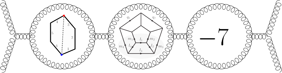
There is a long history of physicists using whimsical animal names for Feynman diagrams, from the penguin to the seagull (no relation). We chose to stick with microscopic organisms: in addition to the tardigrades, we have paramecia and amoebas, even a rogue coccolithophore.

The diagrams we look at have one thing in common, which is key to our proof: the number of lines on the inside of the diagram (“propagators”, which represent “virtual particles”) is related to the number of “loops” in the diagram, as well as the dimension. When these three numbers are related in the right way, it becomes relatively simple to show that any curves we find when computing the Feynman diagram have to be Calabi-Yau.

This includes the most well-known case of Calabi-Yaus showing up in Feynman diagrams, in so-called “banana” or “sunrise” graphs. It’s closely related to some of the cases examined by mathematicians, and our argument ended up pretty close to one made back in 2009 by the mathematician Francis Brown for a different class of diagrams. Oddly enough, neither argument works for the “traintrack” diagrams from our last paper. The tardigrades, paramecia, and amoebas are “more beastly” than those traintracks: their Calabi-Yau curves have more dimensions. In fact, we can show they have the most dimensions possible at each loop, provided all of our particles are massless. In some sense, tardigrades are “as beastly as you can get”.

We still don’t know whether all Feynman diagrams have Calabi-Yau curves, or just these. We’re not even sure how much it matters: it could be that the Calabi-Yau property is a red herring here, noticed because it’s interesting to string theorists but not so informative for us. We don’t understand Calabi-Yaus all that well yet ourselves, so we’ve been looking around at textbooks to try to figure out what people know. One of those textbooks was our inspiration for the “bestiary” in our title, an author whose whimsy we heartily approve of.

Like the classical bestiary, we hope that ours conveys a wholesome moral. There are much stranger beasts in the world of Feynman diagrams than anyone suspected.

IGST 2018

Conference season in Copenhagen continues this week, with Integrability in Gauge and String Theory 2018. Integrability here refers to integrable theories, theories where physicists can calculate things exactly, without the perturbative approximations we typically use. Integrable theories come up in a wide variety of situations, but this conference was focused on the “high-energy” side of the field, on gauge theories (roughly, theories of fundamental forces like Yang-Mills) and string theory.

Integrability is one of the bigger sub-fields in my corner of physics, about the same size as amplitudes. It’s big enough that we can’t host the conference in the old Niels Bohr Institute auditorium.

IMG_20180820_162035401_HDR

Instead, they herded us into the old agriculture school

I don’t normally go to integrability conferences, but when the only cost is bus fare there’s not much to lose. Integrability is arguably amplitudes’s nearest neighbor. The two fields have a history of sharing ideas, and they have similar reputations in the wider community, seen as alternately deep and overly technical. Many of the talks still went over my head, but it was worth getting a chance to see how the neighbors are doing.

Current Themes 2018

I’m at Current Themes in High Energy Physics and Cosmology this week, the yearly conference of the Niels Bohr International Academy. (I talked about their trademark eclectic mix of topics last year.)

This year, the “current theme” was broadly gravitational (though with plenty of exceptions!).

IMG_20180815_180435532

For example, almost getting kicked out of the Botanical Garden

There were talks on phenomena we observe gravitationally, like dark matter. There were talks on calculating amplitudes in gravity theories, both classical and quantum. There were talks about black holes, and the overall shape of the universe. Subir Sarkar talked about his suspicion that the expansion of the universe isn’t actually accelerating, and while I still think the news coverage of it was overblown I sympathize a bit more with his point. He’s got a fairly specific worry, that we’re in a region that’s moving unusually with respect to the surrounding universe, that hasn’t really been investigated in much detail before. I don’t think he’s found anything definitive yet, but it will be interesting as more data accumulates to see what happens.

Of course, current themes can’t stick to just one theme, so there were non-gravitational talks as well. Nima Arkani-Hamed’s talk covered some results he’s talked about in the past, a geometric picture for constraining various theories, but with an interesting new development: while most of the constraints he found restrict things to be positive, one type of constraint he investigated allowed for a very small negative region, around thirty orders of magnitude smaller than the positive part. The extremely small size of the negative region was the most surprising part of the story, as it’s quite hard to get that kind of extremely small scale out of the math we typically invoke in physics (a similar sense of surprise motivates the idea of “naturalness” in particle physics).

There were other interesting talks, which I might talk about later. They should have slides up online soon in case any of you want to have a look.

Different Fields, Different Worlds

My grandfather is a molecular biologist. When we meet, we swap stories: the state of my field and his, different methods and focuses but often a surprising amount of common ground.

Recently he forwarded me an article by Raymond Goldstein, a biological physicist, arguing that biologists ought to be more comfortable with physical reasoning. The article is interesting in its own right, contrasting how physicists and biologists think about the relationship between models, predictions, and experiments. But what struck me most about the article wasn’t the content, but the context.

Goldstein’s article focuses on a question that seemed to me oddly myopic: should physical models be in the Results section, or the Discussion section?

As someone who has never written a paper with either a Results section or a Discussion section, I wondered why anyone would care. In my field, paper formats are fairly flexible. We usually have an Introduction and a Conclusion, yes, but in between we use however many sections we need to explain what we need to. In contrast, biology papers seem to have a very fixed structure: after the Introduction, there’s a Results section, a Discussion section, and a Materials and Methods section at the end.

At first blush, this seemed incredibly bizarre. Why describe your results before the methods you used to get them? How do you talk about your results without discussing them, but still take a full section to do it? And why do reviewers care how you divide things up in the first place?

It made a bit more sense once I thought about how biology differs from theoretical physics. In theoretical physics, the “methods” are most of the result: unsolved problems are usually unsolved because existing methods don’t solve them, and we need to develop new methods to make progress. Our “methods”, in turn, are often the part of the paper experts are most eager to read. In biology, in contrast, the methods are much more standardized. While papers will occasionally introduce new methods, there are so many unexplored biological phenomena that most of the time researchers don’t need to invent a new method: just asking a question no-one else has asked can be enough for a discovery. In that environment, the “results” matter a lot more: they’re the part that takes the most scrutiny, that needs to stand up on its own.

I can even understand the need for a fixed structure. Biology is a much bigger field than theoretical physics. My field is small enough that we all pretty much know each other. If a paper is hard to read, we’ll probably get a chance to ask the author what they meant. Biology, in contrast, is huge. An important result could come from anywhere, and anyone. Having a standardized format makes it a lot easier to scan through an unfamiliar paper and find what you need, especially when there might be hundreds of relevant papers.

The problem with a standardized system, as always, is the existence of exceptions. A more “physics-like” biology paper is more readable with “physics-like” conventions, even if the rest of the field needs to stay “biology-like”. Because of that, I have a lot of sympathy for Goldstein’s argument, but I can’t help but feel that he should be asking for more. If creating new mathematical models and refining them with observation is at the heart of what Goldstein is doing, then maybe he shouldn’t have to use Results/Discussion/Methods in the first place. Maybe he should be allowed to write biology papers that look more like physics papers.

Adversarial Collaborations for Physics

Sometimes physics debates get ugly. For the scientists reading this, imagine your worst opponents. Think of the people who always misinterpret your work while using shoddy arguments to prop up their own, where every question at a talk becomes a screaming match until you just stop going to the same conferences at all.

Now, imagine writing a paper with those people.

Adversarial collaborations, subject of a recent a contest on the blog Slate Star Codex, are a proposed method for resolving scientific debates. Two scientists on opposite sides of an argument commit to writing a paper together, describing the overall state of knowledge on the topic. For the paper to get published, both sides have to sign off on it: they both have to agree that everything in the paper is true. This prevents either side from cheating, or from coming back later with made-up objections: if a point in the paper is wrong, one side or the other is bound to catch it.

This won’t work for the most vicious debates, when one (or both) sides isn’t interested in common ground. But for some ongoing debates in physics, I think this approach could actually help.

One advantage of adversarial collaborations is in preventing accusations of bias. The debate between dark matter and MOND-like proposals is filled with these kinds of accusations: claims that one group or another is ignoring important data, being dishonest about the parameters they need to fit, or applying standards of proof they would never require of their own pet theory. Adversarial collaboration prevents these kinds of accusations: whatever comes out of an adversarial collaboration, both sides would make sure the other side didn’t bias it.

Another advantage of adversarial collaborations is that they make it much harder for one side to move the goalposts, or to accuse the other side of moving the goalposts. From the sidelines, one thing that frustrates me watching string theorists debate whether the theory can describe de Sitter space is that they rarely articulate what it would take to decisively show that a particular model gives rise to de Sitter. Any conclusion of an adversarial collaboration between de Sitter skeptics and optimists would at least guarantee that both parties agreed on the criteria. Similarly, I get the impression that many debates about interpretations of quantum mechanics are bogged down by one side claiming they’ve closed off a loophole with a new experiment, only for the other to claim it wasn’t the loophole they were actually using, something that could be avoided if both sides were involved in the experiment from the beginning.

It’s possible, even likely, that no-one will try adversarial collaboration for these debates. Even if they did, it’s quite possible the collaborations wouldn’t be able to agree on anything! Still, I have to hope that someone takes the plunge and tries writing a paper with their enemies. At minimum, it’ll be an interesting read!

Strings 2018

I’m at Strings this week, in tropical Okinawa. Opening the conference, organizer Hirosi Ooguri joked that they had carefully scheduled things for a sunny time of year, and since the rainy season had just ended “who says that string theorists don’t make predictions?”

IMG_20180625_125441806

There was then a rainstorm during lunch, falsifying string theory

This is the first time I’ve been to Strings. There are almost 500 people here, which might seem small for folks in other fields, but for me this is the biggest conference I’ve attended. The size is noticeable in the little things: this is the first conference I’ve been to with a diaper changing room, the first managed by a tour company, the first with a dedicated “Cultural Evening” featuring classical music from the region. With this in mind, the conference were impressively well-organized, but there were some substantial gaps (tightly packed tours before the Cultural Evening that didn’t leave time for dinner, and a talk by Morrison cut short by missing slides that offset the schedule of the whole last day).

On the well-organized side, Strings has a particular structure for its talks, with Review Talks and Plenary Talks. The Review Talks each summarize a subject: mostly main focuses of the conference, but with a few (Ashoke Sen on String Field Theory, David Simmons-Duffin on the Conformal Bootstrap) that only covered the content of a few talks.

I’m not going to make another pie chart this year, if you want that kind of breakdown Daniel Harlow gave one during the “Golden Jubilee” at the end. If I did something like that this time, I’d divide it up not by sub-fields, but by goals. Talks here focused on a few big questions: “Can we classify all quantum field theories?” “What are the general principles behind quantum gravity?” “Can we make some of the murky aspects of string theory clearer?” “How can string theory give rise to sensible physics in four dimensions?”

Of those questions, classifying quantum field theories made up the bulk of the conference. I’ve heard people dismiss this work on the ground that much of it only works in supersymmetric theories. With that in mind, it was remarkable just how much of the conference was non-supersymmetric. Supersymmetry still played a role, but the assumption seemed to be that it was more of a sub-topic than something universal (to the extent that one of the Review Talks, Clay Cordova’s “What’s new with Q?”, was “the supersymmetry review talk”). Both supersymmetric and non-supersymmetric theories are increasingly understood as being part of a “landscape”, linked by duality and thinking at different scales. These links are sometimes understood in terms of string theory, but often not. So far it’s not clear if there is a real organizing principle here, especially for the non-supersymmetric cases, and people seem to be kept busy enough just proving the links they observe.

Finding general principles behind quantum gravity motivated a decent range of the talks, from Andrew Strominger to Jorge Santos. The topics that got the most focus, and two of the Review Talks, were by what I’ve referred to as “entanglers”, people investigating the structure of space and time via quantum entanglement and entropy. My main takeaway from these talks was perhaps a bit frivolous: between Maldacena’s talk (about an extremely small wormhole made from Standard Model-compatible building blocks) and Hartman’s discussion of the Average Null Energy Condition, it looks like a “useful sci-fi wormhole” (specifically, one that gets you there faster than going the normal way) has been conclusively ruled out in quantum field theory.

Only a minority of talks discussed using string theory to describe the real world, though I get the impression this was still more focus than in past years. In particular, there were several talks trying to discover properties of Calabi-Yaus, the geometries used to curl up string theory’s extra dimensions. Watching these talks I had a similar worry to Strominger’s question after Irene Valenzuela’s talk: it’s not clear that these investigations aren’t just examining a small range of possibilities, one that might become irrelevant if new dualities or types of compactification are found. Ironically, this objection seems to apply least to Valenzuela’s talk itself: characterizing the “swampland” of theories that don’t make sense as part of a theory of quantum gravity may start with examples from string compactifications, but its practitioners are looking for more general principles about quantum gravity and seem to manage at least reasonable arguments that don’t depend on string theory being true.

There wasn’t much from the amplitudes field at this conference, with just Yu-tin Huang’s talk carrying that particular flag. Despite that, amplitudes methods came up in several talks, with Silviu Pufu praising an amplitudes textbook and David Simmons-Duffin bringing up amplitudes several times (more than he did in his talk last week at Amplitudes).

The end of the conference featured a panel discussion in honor of String Theory’s 50th Anniversary, its “Golden Jubilee”. The panel was evenly split between founders of string theory, heroes of the string duality revolution, and the current crop of young theorists. The panelists started by each giving a short presentation. Michael Green joked that it felt like a “geriatric gong show”, and indeed a few of the presentations were gong show-esque. Still, some of the speeches were inspiring. I was particularly impressed by Juan Maldacena, Eva Silverstein, and Daniel Harlow, who each laid out a compelling direction for string theory’s future. The questions afterwards were collated by David Gross from audience submissions, and were largely what you would expect, with quite a lot of questions about whether string theory can ever connect with experiment. I was more than a little disappointed by the discussion of whether string theory can give rise to de Sitter space, which was rather botched: Maldacena was appointed as the defender of de Sitter, but (contra Gross’s summary) the quantum complexity-based derivation he proposed didn’t sound much like the flux compactifications that have inspired so much controversy, so everyone involved ended up talking past each other.

Edit: See Shamit’s comment below, I apparently misunderstood what Maldacena was referring to.

Amplitudes 2018

This week, I’m at Amplitudes, my field’s big yearly conference. The conference is at SLAC National Accelerator Laboratory this year, a familiar and lovely place.

IMG_20180620_183339441_HDR

Welcome to the Guest House California

It’s been a packed conference, with a lot of interesting talks. Recording and slides of most of them should be up at this point, for those following at home. I’ll comment on a few that caught my attention, I might do a more in-depth post later.

The first morning was dedicated to gravitational waves. At the QCD Meets Gravity conference last December I noted that amplitudes folks were very eager to do something relevant to LIGO, but that it was still a bit unclear how we could contribute (aside from Pierpaolo Mastrolia, who had already figured it out). The following six months appear to have cleared things up considerably, and Clifford Cheung and Donal O’Connel’s talks laid out quite concrete directions for this kind of research.

I’d seen Erik Panzer talk about the Hepp bound two weeks ago at Les Houches, but that was for a much more mathematically-inclined audience. It’s been interesting seeing people here start to see the implications: a simple method to classify and estimate (within 1%!) Feynman integrals could be a real game-changer.

Brenda Penante’s talk made me rethink a slogan I like to quote, that N=4 super Yang-Mills is the “most transcendental” part of QCD. While this is true in some cases, in many ways it’s actually least true for amplitudes, with quite a few counterexamples. For other quantities (like the form factors that were the subject of her talk) it’s true more often, and it’s still unclear when we should expect it to hold, or why.

Nima Arkani-Hamed has a reputation for talks that end up much longer than scheduled. Lately, it seems to be due to the sheer number of projects he’s working on. He had to rush at the end of his talk, which would have been about cosmological polytopes. I’ll have to ask his collaborator Paolo Benincasa for an update when I get back to Copenhagen.

Tuesday afternoon was a series of talks on the “NNLO frontier”, two-loop calculations that form the state of the art for realistic collider physics predictions. These talks brought home to me that the LHC really does need two-loop precision, and that the methods to get it are still pretty cumbersome. For those of us off in the airy land of six-loop N=4 super Yang-Mills, this is the challenge: can we make what these people do simpler?

Wednesday cleared up a few things for me, from what kinds of things you can write down in “fishnet theory” to how broad Ashoke Sen’s soft theorem is, to how fast John Joseph Carrasco could show his villanelle slide. It also gave me a clearer idea of just what simplifications are available for pushing to higher loops in supergravity.

Wednesday was also the poster session. It keeps being amazing how fast the field is growing, the sheer number of new faces was quite inspiring. One of those new faces pointed me to a paper I had missed, suggesting that elliptic integrals could end up trickier than most of us had thought.

Thursday featured two talks by people who work on the Conformal Bootstrap, one of our subfield’s closest relatives. (We’re both “bootstrappers” in some sense.) The talks were interesting, but there wasn’t a lot of engagement from the audience, so if the intent was to make a bridge between the subfields I’m not sure it panned out. Overall, I think we’re mostly just united by how we feel about Simon Caron-Huot, who David Simmons-Duffin described as “awesome and mysterious”. We also had an update on attempts to extend the Pentagon OPE to ABJM, a three-dimensional analogue of N=4 super Yang-Mills.

I’m looking forward to Friday’s talks, promising elliptic functions among other interesting problems.

Quelques Houches

For the last two weeks I’ve been at Les Houches, a village in the French Alps, for the Summer School on Structures in Local Quantum Field Theory.

IMG_20180614_104537425

To assist, we have a view of some very large structures in local quantum field theory

Les Houches has a long history of prestigious summer schools in theoretical physics, going back to the activity of Cécile DeWitt-Morette after the second world war. This was more of a workshop than a “school”, though: each speaker gave one talk, and they weren’t really geared for students.

The workshop was organized by Dirk Kreimer and Spencer Bloch, who both have a long track record of work on scattering amplitudes with a high level of mathematical sophistication. The group they invited was an even mix of physicists interested in mathematics and mathematicians interested in physics. The result was a series of talks that managed to both be thoroughly technical and ask extremely deep questions, including “is quantum electrodynamics really an asymptotic series?”, “are there simple graph invariants that uniquely identify Feynman integrals?”, and several talks about something called the Spine of Outer Space, which still sounds a bit like a bad sci-fi novel. Along the way there were several talks showcasing the growing understanding of elliptic polylogarithms, giving me an opportunity to quiz Johannes Broedel about his recent work.

While some of the more mathematical talks went over my head, they spurred a lot of productive dialogues between physicists and mathematicians. Several talks had last-minute slides, added as a result of collaborations that happened right there at the workshop. There was even an entire extra talk, by David Broadhurst, based on work he did just a few days before.

We also had a talk by Jaclyn Bell, a former student of one of the participants who was on a BBC reality show about training to be an astronaut. She’s heavily involved in outreach now, and honestly I’m a little envious of how good she is at it.

An Omega for Every Alpha

In particle physics, we almost always use approximations.

Often, we assume the forces we consider are weak. We use a “coupling constant”, some number written g or a or \alpha, and we assume it’s small, so \alpha is greater than \alpha^2 is greater than \alpha^3. With this assumption, we can start drawing Feynman diagrams, and each “loop” we add to the diagram gives us a higher power of \alpha.

If \alpha isn’t small, then the trick stops working, the diagrams stop making sense, and we have to do something else.

Except for some times, when everything keeps working fine. This week, along with Simon Caron-Huot, Lance Dixon, Andrew McLeod, and Georgios Papathanasiou, I published what turned out to be a pretty cute example.

omegapic

We call this fellow \Omega. It’s a family of diagrams that we can write down for any number of loops: to get more loops, just extend the “…”, adding more boxes in the middle. Count the number of lines sticking out, and you get six: these are “hexagon functions”, the type of function I’ve used to calculate six-particle scattering in N=4 super Yang-Mills.

The fun thing about \Omega is that we don’t have to think about it this way, one loop at a time. We can add up all the loops, \alpha times one loop plus \alpha^2 times two loops plus \alpha^3 times three loops, all the way up to infinity. And we’ve managed to figure out what those loops sum to.

omegaeqnpic

The result ends up beautifully simple. This formula isn’t just true for small coupling constants, it’s true for any number you care to plug in, making the forces as strong as you’d like.

We can do this with \Omega because we have equations relating different loops together. Solving those equations with a few educated guesses, we can figure out the full sum. We can also go back, and use those equations to take the \Omegas at each loop apart, finding a basis of functions needed to describe them.

That basis is the real reward here. It’s not the full basis of “hexagon functions”: if you wanted to do a full six-particle calculation, you’d need more functions than the ones \Omega is made of. What it is, though, is a basis we can describe completely, stating exactly what it’s made of for any number of loops.

We can’t do that with the hexagon functions, at least not yet: we have to build them loop by loop, one at a time before we can find the next ones. The hope, though, is that we won’t have to do this much longer. The \Omega basis covers some of the functions we need. Our hope is that other nice families of diagrams can cover the rest. If we can identify more functions like \Omega, things that we can sum to any number of loops, then perhaps we won’t have to think loop by loop anymore. If we know the right building blocks, we might be able to guess the whole amplitude, to find a formula that works for any \alpha you’d like.

That would be a big deal. N=4 super Yang-Mills isn’t the real world, but it’s complicated in some of the same ways. If we can calculate there without approximations, it should at least give us an idea of what part of the real-world answer can look like. And for a field that almost always uses approximations, that’s some pretty substantial progress.

Be Rational, Integrate Our Way!

I’ve got another paper up this week with Jacob Bourjaily, Andrew McLeod, and Matthias Wilhelm, about integrating Feynman diagrams.

If you’ve been following this blog for a while, you might be surprised: most of my work avoids Feynman diagrams at all costs. I’ve changed my mind, in part, because it turns out integrating Feynman diagrams can be a lot easier than I had thought.

At first, I thought Feynman integrals would be hard purely because they’re integrals. Those of you who’ve taken calculus might remember that, while taking derivatives was just a matter of following the rules, doing integrals required a lot more thought. Rather than one set of instructions, you had a set of tricks, meant to try to match your integral to the derivative of some known function. Sometimes the tricks worked, sometimes you just ended up completely lost.

As it turns out, that’s not quite the problem here. When I integrate a Feynman diagram, most of the time I’m expecting a particular kind of result, called a polylogarithm. If you know that’s the end goal, then you really can just follow the rules, using partial-fractioning to break your integral up into simpler integrations, linear pieces that you can match to the definition of polylogarithms. There are even programs that do this for you: Erik Panzer’s HyperInt is an especially convenient one.

maplewhining

Or it would be convenient, if Maple’s GUI wasn’t cursed…

Still, I wouldn’t have expected Feynman integrals to work particularly well, because they require too many integrations. You need to integrate a certain number of times to define a polylogarithm: for the ones we get out of Feynman diagrams, it’s two integrations for each loop the diagram has. The usual ways we calculate Feynman diagrams lead to a lot more integrations: the systematic method, using something called Symanzik polynomials, involves one integration per particle line in the diagram, which usually adds up to a lot more than two per loop.

When I arrived at the Niels Bohr Institute, I assumed everyone in my field knew about Symanzik polynomials. I was surprised when it turned out Jake Bourjaily hadn’t even heard of them. He was integrating Feynman diagrams by what seemed like a plodding, unsystematic method, taking the intro example from textbooks and just applying it over and over, gaining no benefit from all of the beautiful graph theory that goes into the Symanzik polynomials.

I was even more surprised when his method turned out to be the better one.

Avoid Symanzik polynomials, and you can manage with a lot fewer integrations. Suddenly we were pretty close to the “two integrations per loop” sweet spot, with only one or two “extra” integrations to do.

A few more advantages, and Feynman integrals were actually looking reasonable. The final insight came when we realized that just writing the problem in the right variables made a huge difference.

HyperInt, as I mentioned, tries to break a problem up into simpler integrals. Specifically, it’s trying to make things linear in the integration variable. In order to do this, sometimes it has to factor quadratic polynomials, like so:

partialfractionformula

Notice the square roots in this formula? Those can make your life a good deal trickier. Once you’ve got irrational functions in the game, HyperInt needs extra instructions for how to handle them, and integration is a lot more cumbersome.

The last insight, then, and the key point in our paper, is to avoid irrational functions. To do that, we use variables that rationalize the square roots.

We get these variables from one of the mainstays of our field, called momentum twistors. These variables are most useful in our favorite theory of N=4 super Yang-Mills, but they’re useful in other contexts too. By parametrizing them with a good “chart”, one with only the minimum number of variables we need to capture the integral, we can rationalize most of the square roots we encounter.

That “most” is going to surprise some people. We rationalized all of the expected square roots, letting us do integrals all the way to four loops in a few cases. But there were some unexpected square roots, and those we couldn’t rationalize.

These unexpected square roots don’t just make our life more complicated, if they stick around in a physically meaningful calculation they’ll upset a few other conjectures as well. People had expected that these integrals were made of certain kinds of “letters”, organized by a mathematical structure called a cluster algebra. That cluster algebra structure doesn’t have room for square roots, which suggests that it can’t be the full story here.

The integrals that we can do, though, with no surprise square roots? They’re much easier than anyone expected, much easier than with any other method. Rather than running around doing something fancy, we just integrated things the simple, rational way…and it worked!