Tag Archives: theoretical physics

Quelques Houches

For the last two weeks I’ve been at Les Houches, a village in the French Alps, for the Summer School on Structures in Local Quantum Field Theory.

IMG_20180614_104537425

To assist, we have a view of some very large structures in local quantum field theory

Les Houches has a long history of prestigious summer schools in theoretical physics, going back to the activity of Cécile DeWitt-Morette after the second world war. This was more of a workshop than a “school”, though: each speaker gave one talk, and they weren’t really geared for students.

The workshop was organized by Dirk Kreimer and Spencer Bloch, who both have a long track record of work on scattering amplitudes with a high level of mathematical sophistication. The group they invited was an even mix of physicists interested in mathematics and mathematicians interested in physics. The result was a series of talks that managed to both be thoroughly technical and ask extremely deep questions, including “is quantum electrodynamics really an asymptotic series?”, “are there simple graph invariants that uniquely identify Feynman integrals?”, and several talks about something called the Spine of Outer Space, which still sounds a bit like a bad sci-fi novel. Along the way there were several talks showcasing the growing understanding of elliptic polylogarithms, giving me an opportunity to quiz Johannes Broedel about his recent work.

While some of the more mathematical talks went over my head, they spurred a lot of productive dialogues between physicists and mathematicians. Several talks had last-minute slides, added as a result of collaborations that happened right there at the workshop. There was even an entire extra talk, by David Broadhurst, based on work he did just a few days before.

We also had a talk by Jaclyn Bell, a former student of one of the participants who was on a BBC reality show about training to be an astronaut. She’s heavily involved in outreach now, and honestly I’m a little envious of how good she is at it.

An Omega for Every Alpha

In particle physics, we almost always use approximations.

Often, we assume the forces we consider are weak. We use a “coupling constant”, some number written g or a or \alpha, and we assume it’s small, so \alpha is greater than \alpha^2 is greater than \alpha^3. With this assumption, we can start drawing Feynman diagrams, and each “loop” we add to the diagram gives us a higher power of \alpha.

If \alpha isn’t small, then the trick stops working, the diagrams stop making sense, and we have to do something else.

Except for some times, when everything keeps working fine. This week, along with Simon Caron-Huot, Lance Dixon, Andrew McLeod, and Georgios Papathanasiou, I published what turned out to be a pretty cute example.

omegapic

We call this fellow \Omega
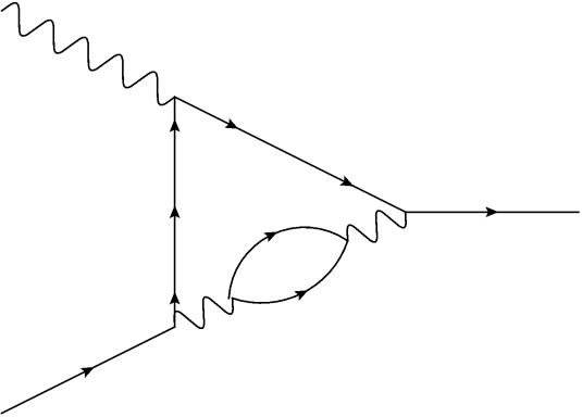
. It’s a family of diagrams that we can write down for any number of loops: to get more loops, just extend the “…”, adding more boxes in the middle. Count the number of lines sticking out, and you get six: these are “hexagon functions”, the type of function I’ve used to calculate six-particle scattering in N=4 super Yang-Mills.

The fun thing about \Omega is that we don’t have to think about it this way, one loop at a time. We can add up all the loops, \alpha times one loop plus \alpha^2 times two loops plus \alpha^3 times three loops, all the way up to infinity. And we’ve managed to figure out what those loops sum to.

omegaeqnpic

The result ends up beautifully simple. This formula isn’t just true for small coupling constants, it’s true for any number you care to plug in, making the forces as strong as you’d like.

We can do this with \Omega because we have equations relating different loops together. Solving those equations with a few educated guesses, we can figure out the full sum. We can also go back, and use those equations to take the \Omegas at each loop apart, finding a basis of functions needed to describe them.

That basis is the real reward here. It’s not the full basis of “hexagon functions”: if you wanted to do a full six-particle calculation, you’d need more functions than the ones \Omega is made of. What it is, though, is a basis we can describe completely, stating exactly what it’s made of for any number of loops.

We can’t do that with the hexagon functions, at least not yet: we have to build them loop by loop, one at a time before we can find the next ones. The hope, though, is that we won’t have to do this much longer. The \Omega basis covers some of the functions we need. Our hope is that other nice families of diagrams can cover the rest. If we can identify more functions like \Omega, things that we can sum to any number of loops, then perhaps we won’t have to think loop by loop anymore. If we know the right building blocks, we might be able to guess the whole amplitude, to find a formula that works for any \alpha you’d like.

That would be a big deal. N=4 super Yang-Mills isn’t the real world, but it’s complicated in some of the same ways. If we can calculate there without approximations, it should at least give us an idea of what part of the real-world answer can look like. And for a field that almost always uses approximations, that’s some pretty substantial progress.

Be Rational, Integrate Our Way!

I’ve got another paper up this week with Jacob Bourjaily, Andrew McLeod, and Matthias Wilhelm, about integrating Feynman diagrams.

If you’ve been following this blog for a while, you might be surprised: most of my work avoids Feynman diagrams at all costs. I’ve changed my mind, in part, because it turns out integrating Feynman diagrams can be a lot easier than I had thought.

At first, I thought Feynman integrals would be hard purely because they’re integrals. Those of you who’ve taken calculus might remember that, while taking derivatives was just a matter of following the rules, doing integrals required a lot more thought. Rather than one set of instructions, you had a set of tricks, meant to try to match your integral to the derivative of some known function. Sometimes the tricks worked, sometimes you just ended up completely lost.

As it turns out, that’s not quite the problem here. When I integrate a Feynman diagram, most of the time I’m expecting a particular kind of result, called a polylogarithm. If you know that’s the end goal, then you really can just follow the rules, using partial-fractioning to break your integral up into simpler integrations, linear pieces that you can match to the definition of polylogarithms. There are even programs that do this for you: Erik Panzer’s HyperInt is an especially convenient one.

maplewhining

Or it would be convenient, if Maple’s GUI wasn’t cursed…

Still, I wouldn’t have expected Feynman integrals to work particularly well, because they require too many integrations. You need to integrate a certain number of times to define a polylogarithm: for the ones we get out of Feynman diagrams, it’s two integrations for each loop the diagram has. The usual ways we calculate Feynman diagrams lead to a lot more integrations: the systematic method, using something called Symanzik polynomials, involves one integration per particle line in the diagram, which usually adds up to a lot more than two per loop.

When I arrived at the Niels Bohr Institute, I assumed everyone in my field knew about Symanzik polynomials. I was surprised when it turned out Jake Bourjaily hadn’t even heard of them. He was integrating Feynman diagrams by what seemed like a plodding, unsystematic method, taking the intro example from textbooks and just applying it over and over, gaining no benefit from all of the beautiful graph theory that goes into the Symanzik polynomials.

I was even more surprised when his method turned out to be the better one.

Avoid Symanzik polynomials, and you can manage with a lot fewer integrations. Suddenly we were pretty close to the “two integrations per loop” sweet spot, with only one or two “extra” integrations to do.

A few more advantages, and Feynman integrals were actually looking reasonable. The final insight came when we realized that just writing the problem in the right variables made a huge difference.

HyperInt, as I mentioned, tries to break a problem up into simpler integrals. Specifically, it’s trying to make things linear in the integration variable. In order to do this, sometimes it has to factor quadratic polynomials, like so:

partialfractionformula

Notice the square roots in this formula? Those can make your life a good deal trickier. Once you’ve got irrational functions in the game, HyperInt needs extra instructions for how to handle them, and integration is a lot more cumbersome.

The last insight, then, and the key point in our paper, is to avoid irrational functions. To do that, we use variables that rationalize the square roots.

We get these variables from one of the mainstays of our field, called momentum twistors. These variables are most useful in our favorite theory of N=4 super Yang-Mills, but they’re useful in other contexts too. By parametrizing them with a good “chart”, one with only the minimum number of variables we need to capture the integral, we can rationalize most of the square roots we encounter.

That “most” is going to surprise some people. We rationalized all of the expected square roots, letting us do integrals all the way to four loops in a few cases. But there were some unexpected square roots, and those we couldn’t rationalize.

These unexpected square roots don’t just make our life more complicated, if they stick around in a physically meaningful calculation they’ll upset a few other conjectures as well. People had expected that these integrals were made of certain kinds of “letters”, organized by a mathematical structure called a cluster algebra. That cluster algebra structure doesn’t have room for square roots, which suggests that it can’t be the full story here.

The integrals that we can do, though, with no surprise square roots? They’re much easier than anyone expected, much easier than with any other method. Rather than running around doing something fancy, we just integrated things the simple, rational way…and it worked!

Calabi-Yaus for Higgs Phenomenology

less joking title:

You Didn’t Think We’d Stop at Elliptics, Did You?

When calculating scattering amplitudes, I like to work with polylogarithms. They’re a very well-understood type of mathematical function, and thus pretty easy to work with.

Even for our favorite theory of N=4 super Yang-Mills, though, they’re not the whole story. You need other types of functions to represent amplitudes, elliptic polylogarithms that are only just beginning to be properly understood. We had our own modest contribution to that topic last year.

You can think of the difference between these functions in terms of more and more complicated curves. Polylogarithms just need circles or spheres, elliptic polylogarithms can be described with a torus.

A torus is far from the most complicated curve you can think of, though.

983px-calabi_yau_formatted-svgString theorists have done a lot of research into complicated curves, in particular ones with a property called Calabi-Yau. They were looking for ways to curl up six or seven extra dimensions, to get down to the four we experience. They wanted to find ways of curling that preserved some supersymmetry, in the hope that they could use it to predict new particles, and it turned out that Calabi-Yau was the condition they needed.

That hope, for the most part, didn’t pan out. There were too many Calabi-Yaus to check, and the LHC hasn’t seen any supersymmetric particles. Today, “string phenomenologists”, who try to use string theory to predict new particles, are a relatively small branch of the field.

This research did, however, have lasting impact: due to string theorists’ interest, there are huge databases of Calabi-Yau curves, and fruitful dialogues with mathematicians about classifying them.

This has proven quite convenient for us, as we happen to have some Calabi-Yaus to classify.

traintrackpic

Our midnight train going anywhere…in the space of Calabi-Yaus

We call Feynman diagrams like the one above “traintrack integrals”. With two loops, it’s the elliptic integral we calculated last year. With three, though, you need a type of Calabi-Yau curve called a K3. With four loops, it looks like you start needing Calabi-Yau three-folds, the type of space used to compactify string theory to four dimensions.

“We” in this case is myself, Jacob Bourjaily, Andrew McLeod, Matthias Wilhelm, and Yang-Hui He, a Calabi-Yau expert we brought on to help us classify these things. Our new paper investigates these integrals, and the more and more complicated curves needed to compute them.

Calabi-Yaus had been seen in amplitudes before, in diagrams called “sunrise” or “banana” integrals. Our example shows that they should occur much more broadly. “Traintrack” integrals appear in our favorite N=4 super Yang-Mills theory, but they also appear in theories involving just scalar fields, like the Higgs boson. For enough loops and particles, we’re going to need more and more complicated functions, not just the polylogarithms and elliptic polylogarithms that people understand.

(And to be clear, no, nobody needs to do this calculation for Higgs bosons in practice. This diagram would calculate the result of two Higgs bosons colliding and producing ten or more Higgs bosons, all at energies so high you can ignore their mass, which is…not exactly relevant for current collider phenomenology. Still, the title proved too tempting to resist.)

Is there a way to understand traintrack integrals like we understand polylogarithms? What kinds of Calabi-Yaus do they pick out, in the vast space of these curves? We’d love to find out. For the moment, we just wanted to remind all the people excited about elliptic polylogarithms that there’s quite a bit more strangeness to find, even if we don’t leave the tracks.

The State of Four Gravitons

This blog is named for a question: does the four-graviton amplitude in N=8 supergravity diverge?

Over the years, Zvi Bern and a growing cast of collaborators have been trying to answer that question. They worked their way up, loop by loop, until they stalled at five loops. Last year, they finally broke the stall, and last week, they published the result of the five-loop calculation. They find that N=8 supergravity does not diverge at five loops in four dimensions, but does diverge in 24/5 dimensions. I thought I’d write a brief FAQ about the status so far.

Q: Wait a minute, 24/5 dimensions? What does that mean? Are you talking about fractals, or…

Nothing so exotic. The number 24/5 comes from a regularization trick. When we’re calculating an amplitude that might be divergent, one way to deal with it is to treat the dimension like a free variable. You can then see what happens as you vary the dimension, and see when the amplitude starts diverging. If the dimension is an integer, then this ends up matching a more physics-based picture, where you start with a theory in eleven dimensions and curl up the extra ones until you get to the dimension you’re looking for. For fractional dimensions, it’s not clear that there’s any physical picture like this: it’s just a way to talk about how close something is to diverging.

Q: I’m really confused. What’s a graviton? What is supergravity? What’s a divergence?

I don’t have enough space to explain these things here, but that’s why I write handbooks. Here are explanations of gravitons, supersymmetry, and (N=8) supergravity, loops, and divergences. Please let me know if anything in those explanations is unclear, or if you have any more questions.

Q: Why do people think that N=8 supergravity will diverge at seven loops?

There’s a useful rule of thumb in quantum field theory: anything that can happen, will happen. In this case, that means if there’s a way for a theory to diverge that’s consistent with the symmetries of the theory, then it almost always does diverge. In the past, that meant that people expected N=8 supergravity to diverge at five loops. However, researchers found a previously unknown symmetry that looked like it would forbid the five-loop divergence, and only allow a divergence at seven loops (in four dimensions). Zvi and co.’s calculation confirms that the five-loop divergence doesn’t show up.

More generally, string theory not only avoids divergences but clears up other phenomena, like black holes. These two things seem tied together: string theory cleans up problems in quantum gravity in a consistent, unified way. There isn’t a clear way for N=8 supergravity on its own to clean up these kinds of problems, which makes some people skeptical that it can match string theory’s advantages. Either way N=8 supergravity, unlike string theory, isn’t a candidate theory of nature by itself: it would need to be modified in order to describe our world, and no-one has suggested a way to do that.

Q: Why do people think that N=8 supergravity won’t diverge at seven loops?

There’s a useful rule of thumb in amplitudes: amplitudes are weird. In studying amplitudes we often notice unexpected simplifications, patterns that uncover new principles that weren’t obvious before.

Gravity in general seems to have a lot of these kinds of simplifications. Even without any loops, its behavior is surprisingly tame: it’s a theory that we can build up piece by piece from the three-particle interaction, even though naively we shouldn’t be able to (for the experts: I’m talking about large-z behavior in BCFW). This behavior seems to have an effect on one-loop amplitudes as well. There are other ways in which gravity seems better-behaved than expected, overall this suggests that we still have a fair ways to go before we understand all of the symmetries of gravity theories.

Supersymmetric gravity in particular also seems unusually well-behaved. N=5 supergravity was expected to diverge at four loops, but doesn’t. N=4 supergravity does diverge at four loops, but that seems to be due to an effect that is specific to that case (for the experts: an anomaly).

For N=8 specifically, a suggestive hint came from varying the dimension. If you checked the dimension in which the theory diverged at each loop, you’d find it matched the divergences of another theory, N=4 super Yang-Mills. At l 
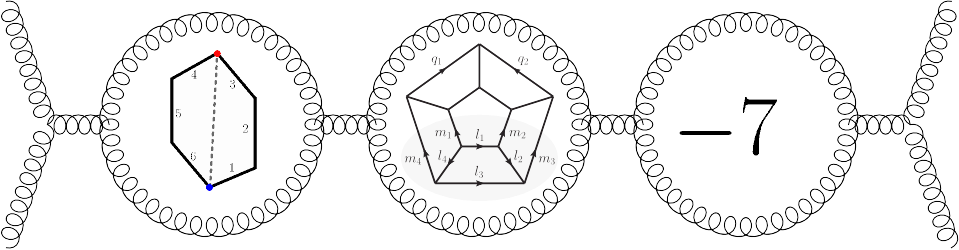
loops, N=4 super Yang-Mills diverges in dimension 4+6/l. From that formula, you can see that no matter how much you increase l, you’ll never get to four dimensions: in four dimensions, N=4 super Yang-Mills doesn’t diverge.

At five loops, N=4 super Yang-Mills diverges in 26/5 dimensions. Zvi Bern made a bet with supergravity expert Kelly Stelle that the dimension would be the same for N=8 supergravity: a bottle of California wine from Bern versus English wine from Stelle. Now that they’ve found a divergence in 24/5 dimensions instead, Stelle will likely be getting his wine soon.

Q: It sounds like the calculation was pretty tough. Can they still make it to seven loops?

I think so, yes. Doing the five-loop calculation they noticed simplifications, clever tricks uncovered by even more clever grad students. The end result is that if they just want to find out whether the theory diverges then they don’t have to do the “whole calculation”, just part of it. This simplifies things a lot. They’ll probably have to find a few more simplifications to make seven loops viable, but I’m optimistic that they’ll find them, and in the meantime the new tricks should have some applications in other theories.

Q: What do you think? Will the theory diverge?

I’m not sure.

To be honest, I’m a bit less optimistic than I used to be. The agreement of divergence dimensions between N=8 supergravity and N=4 super Yang-Mills wasn’t the strongest argument (there’s a reason why, though Stelle accepted the bet on five loops, string theorist Michael Green is waiting on seven loops for his bet). Fractional dimensions don’t obviously mean anything physically, and many of the simplifications in gravity seem specific to four dimensions. Still, it was suggestive, the kind of “motivation” that gets a conjecture started.

Without that motivation, none of the remaining arguments are specific to N=8. I still think unexpected simplifications are likely, that gravity overall behaves better than we yet appreciate. I still would bet on seven loops being finite. But I’m less confident about what it would mean for the theory overall. That’s going to take more serious analysis, digging in to the anomaly in N=4 supergravity and seeing what generalizes. It does at least seem like Zvi and co. are prepared to undertake that analysis.

Regardless, it’s still worth pushing for seven loops. Having that kind of heavy-duty calculation in our sub-field forces us to improve our mathematical technology, in the same way that space programs and particle colliders drive technology in the wider world. If you think your new amplitudes method is more efficient than the alternatives, the push to seven loops is the ideal stress test. Jacob Bourjaily likes to tell me how his prescriptive unitarity technique is better than what Zvi and co. are doing, this is our chance to find out!

Overall, I still stand by what I say in my blog’s sidebar. I’m interested in N=8 supergravity, I’d love to find out whether the four-graviton amplitude diverges…and now that the calculation is once again making progress, I expect that I will.

By Any Other Author Would Smell as Sweet

I was chatting with someone about this paper (which probably deserves a post in its own right, once I figure out an angle that isn’t just me geeking out about how much I could do with their new setup), and I referred to it as “Claude’s paper”. This got me chided a bit: the paper has five authors, experts on Feynman diagrams and elliptic integrals. It’s not just “Claude’s paper”. So why do I think of it that way?

Part of it, I think, comes from the experience of reading a paper. We want to think of a paper as a speech act: someone talking to us, explaining something, leading us through a calculation. Our brain models that as a conversation with a single person, so we naturally try to put a single face to a paper. With a collaborative paper, this is almost never how it was written: different sections are usually written by different people, who then edit each other’s work. But unless you know the collaborators well, you aren’t going to know who wrote which section, so it’s easier to just picture one author for the whole thing.

Another element comes from how I think about the field. Just as it’s easier to think of a paper as the speech of one person, it’s easier to think of new developments as continuations of a story. I at least tend to think about the field in terms of specific programs: these people worked on this, which is a continuation of that. You can follow those kinds of threads though the field, but in reality they’re tangled together: collaborations are an opportunity for two programs to meet. In other fields you might have a “first author” to default to, but in theoretical physics we normally write authors alphabetically. For “Claude’s paper”, it just feels like the sort of thing I’d expect Claude Duhr to write, like a continuation of the other things he’s known for, even if it couldn’t have existed without the other four authors.

You’d worry that associating papers with people like this takes away deserved credit. I don’t think it’s quite that simple, though. In an older post I described this paper as the work of Anastasia Volovich and Mark Spradlin. On some level, that’s still how I think about it. Nevertheless, when I heard that Cristian Vergu was going to be at the Niels Bohr Institute next year, I was excited: we’re hiring one of the authors of GSVV! Even if I don’t think of him immediately when I think of the paper, I think of the paper when I think of him.

That, I think, is more important for credit. If you’re a hiring committee, you’ll start out by seeing names of applicants. It’s important, at that point, that you know what they did, that the authors of important papers stand out, that you assign credit where it’s due. It’s less necessary on the other end, when you’re reading a paper and casually classify it in your head.

Nevertheless, I should be more careful about credit. It’s important to remember that “Claude Duhr’s paper” is also “Johannes Broedel’s paper” and “Falko Dulat’s paper”, “Brenda Penante’s paper” and “Lorenzo Tancredi’s paper”. It gives me more of an appreciation of where it comes from, so I can get back to having fun applying it.

A Paper About Ranking Papers

If you’ve ever heard someone list problems in academia, citation-counting is usually near the top. Hiring and tenure committees want easy numbers to judge applicants with: number of papers, number of citations, or related statistics like the h-index. Unfortunately, these metrics can be gamed, leading to a host of bad practices that get blamed for pretty much everything that goes wrong in science. In physics, it’s not even clear that these statistics tell us anything: papers in our field have been including more citations over time, and for thousand-person experimental collaborations the number of citations and papers don’t really reflect any one person’s contribution.

It’s pretty easy to find people complaining about this. It’s much rarer to find a proposed solution.

That’s why I quite enjoyed Alessandro Strumia and Riccardo Torre’s paper last week, on Biblioranking fundamental physics.

Some of their suggestions are quite straightforward. With the number of citations per paper increasing, it makes sense to divide each paper by the number of citations it contains: it means more to get cited by a paper with ten citations than by a paper with one hundred. Similarly, you could divide credit for a paper among its authors, rather than giving each author full credit.

Some are more elaborate. They suggest using a variant of Google’s PageRank algorithm to rank papers and authors. Essentially, the algorithm imagines someone wandering from paper to paper and tries to figure out which papers are more central to the network. This is apparently an old idea, but by combining it with their normalization by number of citations they eke a bit more mileage from it. (I also found their treatment a bit clearer than the older papers they cite. There are a few more elaborate setups in the literature as well, but they seem to have a lot of free parameters so Strumia and Torre’s setup looks preferable on that front.)

One final problem they consider is that of self-citations, and citation cliques. In principle, you could boost your citation count by citing yourself. While that’s easy to correct for, you could also be one of a small number of authors who cite each other a lot. To keep the system from being gamed in this way, they propose a notion of a “CitationCoin” that counts (normalized) citations received minus (normalized) citations given. The idea is that, just as you can’t make anyone richer just by passing money between your friends without doing anything with it, so a small community can’t earn “CitationCoins” without getting the wider field interested.

There are still likely problems with these ideas. Dividing each paper by its number of authors seems like overkill: a thousand-person paper is not typically going to get a thousand times as many citations. I also don’t know whether there are ways to game this system: since the metrics are based in part on citations given, not just citations received, I worry there are situations where it would be to someone’s advantage to cite others less. I think they manage to avoid this by normalizing by number of citations given, and they emphasize that PageRank itself is estimating something we directly care about: how often people read a paper. Still, it would be good to see more rigorous work probing the system for weaknesses.

In addition to the proposed metrics, Strumia and Torre’s paper is full of interesting statistics about the arXiv and InSpire databases, both using more traditional metrics and their new ones. Whether or not the methods they propose work out, the paper is definitely worth a look.

Why Physicists Leave Physics

It’s an open secret that many physicists end up leaving physics. How many depends on how you count things, but for a representative number, this report has 31% of US physics PhDs in the private sector after one year. I’d expect that number to grow with time post-PhD. While some of these people might still be doing physics, in certain sub-fields that isn’t really an option: it’s not like there are companies that do R&D in particle physics, astrophysics, or string theory. Instead, these physicists get hired in data science, or quantitative finance, or machine learning. Others stay in academia, but stop doing physics: either transitioning to another field, or taking teaching-focused jobs that don’t leave time for research.

There’s a standard economic narrative for why this happens. The number of students grad schools accept and graduate is much higher than the number of professor jobs. There simply isn’t room for everyone, so many people end up doing something else instead.

That narrative is probably true, if you zoom out far enough. On the ground, though, the reasons people leave academia don’t feel quite this “economic”. While they might be indirectly based on a shortage of jobs, the direct reasons matter. Physicists leave physics for a wide variety of reasons, and many of them are things the field could improve on. Others are factors that will likely be present regardless of how many students graduate, or how many jobs there are. I worry that an attempt to address physics attrition on a purely economic level would miss these kinds of details.

I thought I’d talk in this post about a few reasons why physicists leave physics. Most of this won’t be new information to anyone, but I hope some of it is at least a new perspective.

First, to get it out of the way: almost no-one starts a physics PhD with the intention of going into industry. I’ve met a grand total of one person who did, and he’s rather unusual. Almost always, leaving physics represents someone’s dreams not working out.

Sometimes, that just means realizing you aren’t suited for physics. These are people who feel like they aren’t able to keep up with the material, or people who find they aren’t as interested in it as they expected. In my experience, people realize this sort of thing pretty early. They leave in the middle of grad school, or they leave once they have their PhD. In some sense, this is the healthy sort of attrition: without the ability to perfectly predict our interests and abilities, there will always be people who start a career and then decide it’s not for them.

I want to distinguish this from a broader reason to leave, disillusionment. These are people who can do physics, and want to do physics, but encounter a system that seems bent on making them do anything but. Sometimes this means disillusionment with the field itself: phenomenologists sick of tweaking models to lie just beyond the latest experimental bounds, or theorists who had hoped to address the real world but begin to see that they can’t. This kind of motivation lay behind several great atomic physicists going into biology after the second world war, to work on “life rather than death”. Sometimes instead it’s disillusionment with academia: people who have been bludgeoned by academic politics or bureaucracy, who despair of getting the academic system to care about real research or teaching instead of its current screwed-up priorities or who just don’t want to face that kind of abuse again.

When those people leave, it’s at every stage in their career. I’ve seen grad students disillusioned into leaving without a PhD, and successful tenured professors who feel like the field no longer has anything to offer them. While occasionally these people just have a difference of opinion, a lot of the time they’re pointing out real problems with the system, problems that actually should be fixed.

Sometimes, life intervenes. The classic example is the two-body problem, where you and your spouse have trouble finding jobs in the same place. There aren’t all that many places in the world that hire theoretical physicists, and still fewer with jobs open. One or both partners end up needing to compromise, and that can mean switching to a career with a bit more choice in location. People also move to take care of their parents, or because of other connections.

This seems closer to the economic picture, but I don’t think it quite lines up. Even if there were a lot fewer physicists applying for the same number of jobs, it’s still not certain that there’s a job where you want to live, specifically. You’d still end up with plenty of people leaving the field.

A commenter here frequently asks why physicists have to travel so much. Especially for a theorist, why can’t we just work remotely? With current technology, shouldn’t that be pretty easy to do?

I’ve done a lot of remote collaboration, it’s not impossible. But there really isn’t a substitute for working in the same place, for being able to meet someone in the hall and strike up a conversation around a blackboard. Remote collaborations are an ok way to keep a project going, but a rough way to start one. Institutes realize this, which is part of why most of the time they’ll only pay you a salary if they think you’re actually going to show up.

Could I imagine this changing? Maybe. The technology doesn’t exist right now, but maybe someday someone will design a social network with the right features, one where you can strike up and work on collaborations as naturally as you can in person. Then again, maybe I’m silly for imagining a technological solution to the problem in the first place.

What about more direct economic reasons? What about when people leave because of the academic job market itself?

This certainly happens. In my experience though, a lot of the time it’s pre-emptive. You’d think that people would apply for academic jobs, get rejected, and quit the field. More often, I’ve seen people notice the competition for jobs and decide at the outset that it’s not worth it for them. Sometimes this happens right out of grad school. Other times it’s later. In the latter case, these are often people who are “keeping up”, in that their career is moving roughly as fast as everyone else’s. Rather, it’s the stress, of keeping ahead of the field and marketing themselves and applying for every grant in sight and worrying that it could come crashing down any moment, that ends up too much to deal with.

What about the people who do get rejected over and over again?

Physics, like life in Jurassic Park, finds a way. Surprisingly often, these people manage to stick around. Without faculty positions they scrabble up postdoc after postdoc, short-term position after short-term position. They fund their way piece by piece, grant by grant. Often they get depressed, and cynical, and pissed off, and insist that this time they’re just going to quit the field altogether. But from what I’ve seen, once someone is that far in, they often don’t go through with it.

If fewer people went to physics grad school, or more professors were hired, would fewer people leave physics? Yes, absolutely. But there’s enough going on here, enough different causes and different motivations, that I suspect things wouldn’t work out quite as predicted. Some attrition is here to stay, some is independent of the economics. And some, perhaps, is due to problems we ought to actually solve.

Path Integrals and Loop Integrals: Different Things!

When talking science, we need to be careful with our words. It’s easy for people to see a familiar word and assume something totally different from what we intend. And if we use the same word twice, for two different things…

I’ve noticed this problem with the word “integral”. When physicists talk about particle physics, there are two kinds of integrals we mention: path integrals, and loop integrals. I’ve seen plenty of people get confused, and assume that these two are the same thing. They’re not, and it’s worth spending some time explaining the difference.

Let’s start with path integrals (also referred to as functional integrals, or Feynman integrals). Feynman promoted a picture of quantum mechanics in which a particle travels along many different paths, from point A to point B.

three_paths_from_a_to_b

You’ve probably seen a picture like this. Classically, a particle would just take one path, the shortest path, from A to B. In quantum mechanics, you have to add up all possible paths. Most longer paths cancel, so on average the short, classical path is the most important one, but the others do contribute, and have observable, quantum effects. The sum over all paths is what we call a path integral.

It’s easy enough to draw this picture for a single particle. When we do particle physics, though, we aren’t usually interested in just one particle: we want to look at a bunch of different quantum fields, and figure out how they will interact.

We still use a path integral to do that, but it doesn’t look like a bunch of lines from point A to B, and there isn’t a convenient image I can steal from Wikipedia for it. The quantum field theory path integral adds up, not all the paths a particle can travel, but all the ways a set of quantum fields can interact.

How do we actually calculate that?

One way is with Feynman diagrams, and (often, but not always) loop integrals.

4grav2loop

I’ve talked about Feynman diagrams before. Each one is a picture of one possible way that particles can travel, or that quantum fields can interact. In some (loose) sense, each one is a single path in the path integral.

Each diagram serves as instructions for a calculation. We take information about the particles, their momenta and energy, and end up with a number. To calculate a path integral exactly, we’d have to add up all the diagrams we could possibly draw, to get a sum over all possible paths.

(There are ways to avoid this in special cases, which I’m not going to go into here.)

Sometimes, getting a number out of a diagram is fairly simple. If the diagram has no closed loops in it (if it’s what we call a tree diagram) then knowing the properties of the in-coming and out-going particles is enough to know the rest. If there are loops, though, there’s uncertainty: you have to add up every possible momentum of the particles in the loops. You do that with a different integral, and that’s the one that we sometimes refer to as a loop integral. (Perhaps confusingly, these are also often called Feynman integrals: Feynman did a lot of stuff!)

\frac{i^{a+l(1-d/2)}\pi^{ld/2}}{\prod_i \Gamma(a_i)}\int_0^\infty...\int_0^\infty \prod_i\alpha_i^{a_i-1}U^{-d/2}e^{iF/U-i\sum m_i^2\alpha_i}d\alpha_1...d\alpha_n

Loop integrals can be pretty complicated, but at heart they’re the same sort of thing you might have seen in a calculus class. Mathematicians are pretty comfortable with them, and they give rise to numbers that mathematicians find very interesting.

Path integrals are very different. In some sense, they’re an “integral over integrals”, adding up every loop integral you could write down. Mathematicians can define path integrals in special cases, but it’s still not clear that the general case, the overall path integral picture we use, actually makes rigorous mathematical sense.

So if you see physicists talking about integrals, it’s worth taking a moment to figure out which one we mean. Path integrals and loop integrals are both important, but they’re very, very different things.

Writing the Paper Changes the Results

You spent months on your calculation, but finally it’s paid off. Now you just have to write the paper. That’s the easy part, right?

Not quite. Even if writing itself is easy for you, writing a paper is never just writing. To write a paper, you have to make your results as clear as possible, to fit them into one cohesive story. And often, doing that requires new calculations.

It’s something that first really struck me when talking to mathematicians, who may be the most extreme case. For them, a paper needs to be a complete, rigorous proof. Even when they have a result solidly plotted out in their head, when they’re sure they can prove something and they know what the proof needs to “look like”, actually getting the details right takes quite a lot of work.

Physicists don’t have quite the same standards of rigor, but we have a similar paper-writing experience. Often, trying to make our work clear raises novel questions. As we write, we try to put ourselves in the mind of a potential reader. Sometimes our imaginary reader is content and quiet. Other times, though, they object:

“Does this really work for all cases? What about this one? Did you make sure you can’t do this, or are you just assuming? Where does that pattern come from?”

Addressing those objections requires more work, more calculations. Sometimes, it becomes clear we don’t really understand our results at all! The paper takes a new direction, flows with new work to a new, truer message, one we wouldn’t have discovered if we didn’t sit down and try to write it out.