Tag Archives: quantum field theory

Why the Coupling Constants Aren’t Constant: Epistemology and Pragmatism

If you’ve heard a bit about physics, you might have heard that each of the fundamental forces (electromagnetism, the weak nuclear force, the strong nuclear force, and gravity) has a coupling constant, a number, handed down from nature itself, that determines how strong of a force it is. Maybe you’ve seen them in a table, like this:

If you’ve heard a bit more about physics, though, you’ll have heard that those coupling constants aren’t actually constant! Instead, they vary with energy. Maybe you’ve seen them plotted like this:

The usual way physicists explain this is in terms of quantum effects. We talk about “virtual particles”, and explain that any time particles and forces interact, these virtual particles can pop up, adding corrections that change with the energy of the interacting particles. The coupling constant includes all of these corrections, so it can’t be constant, it has to vary with energy.

Maybe you’re happy with this explanation. But maybe you object:

“Isn’t there still a constant, though? If you ignore all the virtual particles, and drop all the corrections, isn’t there some constant number you’re correcting? Some sort of `bare coupling constant’ you could put into a nice table for me?”

There are two reasons I can’t do that. One is an epistemological reason, that comes from what we can and cannot know. The other is practical: even if I knew the bare coupling, most of the time I wouldn’t want to use it.

Let’s start with the epistemology:

The first thing to understand is that we can’t measure the bare coupling directly. When we measure the strength of forces, we’re always measuring the result of quantum corrections. We can’t “turn off” the virtual particles.

You could imagine measuring it indirectly, though. You’d measure the end result of all the corrections, then go back and calculate. That calculation would tell you how big the corrections were supposed to be, and you could subtract them off, solve the equation, and find the bare coupling.

And this would be a totally reasonable thing to do, except that when you go and try to calculate the quantum corrections, instead of something sensible, you get infinity.

We think that “infinity” is due to our ignorance: we know some of the quantum corrections, but not all of them, because we don’t have a final theory of nature. In order to calculate anything we need to hedge around that ignorance, with a trick called renormalization. I talk about that more in an older post. The key message to take away there is that in order to calculate anything we need to give up the hope of measuring certain bare constants, even “indirectly”. Once we fix a few constants that way, the rest of the theory gives reliable predictions.

So we can’t measure bare constants, and we can’t reason our way to them. We have to find the full coupling, with all the quantum corrections, and use that as our coupling constant.

Still, you might wonder, why does the coupling constant have to vary? Can’t I just pick one measurement, at one energy, and call that the constant?

This is where pragmatism comes in. You could fix your constant at some arbitrary energy, sure. But you’ll regret it.

In particle physics, we usually calculate in something called perturbation theory. Instead of calculating something exactly, we have to use approximations. We add up the approximations, order by order, expecting that each time the corrections will get smaller and smaller, so we get closer and closer to the truth.

And this works reasonably well if your coupling constant is small enough, provided it’s at the right energy.

If your coupling constant is at the wrong energy, then your quantum corrections will notice the difference. They won’t just be small numbers anymore. Instead, they end up containing logarithms of the ratio of energies. The more difference between your arbitrary energy scale and the correct one, the bigger these logarithms get.

This doesn’t make your calculation wrong, exactly. It makes your error estimate wrong. It means that your assumption that the next order is “small enough” isn’t actually true. You’d need to go to higher and higher orders to get a “good enough” answer, if you can get there at all.

Because of that, you don’t want to think about the coupling constants as actually constant. If we knew the final theory then maybe we’d know the true numbers, the ultimate bare coupling constants. But we still would want to use coupling constants that vary with energy for practical calculations. We’d still prefer the plot, and not just the table.

A Micrographia of Beastly Feynman Diagrams

5 Replies

Earlier this year, I had a paper about the weird multi-dimensional curves you get when you try to compute trickier and trickier Feynman diagrams. These curves were “Calabi-Yau”, a type of curve string theorists have studied as a way to curl up extra dimensions to preserve something called supersymmetry. At the time, string theorists asked me why Calabi-Yau curves showed up in these Feynman diagrams. Do they also have something to do with supersymmetry?

I still don’t know the general answer. I don’t know if all Feynman diagrams have Calabi-Yau curves hidden in them, or if only some do. But for a specific class of diagrams, I now know the reason. In this week’s paper, with Jacob Bourjaily, Andrew McLeod, and Matthias Wilhelm, we prove it.

We just needed to look at some more exotic beasts to figure it out.

Like this guy!

Meet the tardigrade. In biology, they’re incredibly tenacious microscopic animals, able to withstand the most extreme of temperatures and the radiation of outer space. In physics, we’re using their name for a class of Feynman diagrams.

A clear resemblance!

There is a long history of physicists using whimsical animal names for Feynman diagrams, from the penguin to the seagull (no relation). We chose to stick with microscopic organisms: in addition to the tardigrades, we have paramecia and amoebas, even a rogue coccolithophore.

The diagrams we look at have one thing in common, which is key to our proof: the number of lines on the inside of the diagram (“propagators”, which represent “virtual particles”) is related to the number of “loops” in the diagram, as well as the dimension. When these three numbers are related in the right way, it becomes relatively simple to show that any curves we find when computing the Feynman diagram have to be Calabi-Yau.

This includes the most well-known case of Calabi-Yaus showing up in Feynman diagrams, in so-called “banana” or “sunrise” graphs. It’s closely related to some of the cases examined by mathematicians, and our argument ended up pretty close to one made back in 2009 by the mathematician Francis Brown for a different class of diagrams. Oddly enough, neither argument works for the “traintrack” diagrams from our last paper. The tardigrades, paramecia, and amoebas are “more beastly” than those traintracks: their Calabi-Yau curves have more dimensions. In fact, we can show they have the most dimensions possible at each loop, provided all of our particles are massless. In some sense, tardigrades are “as beastly as you can get”.

We still don’t know whether all Feynman diagrams have Calabi-Yau curves, or just these. We’re not even sure how much it matters: it could be that the Calabi-Yau property is a red herring here, noticed because it’s interesting to string theorists but not so informative for us. We don’t understand Calabi-Yaus all that well yet ourselves, so we’ve been looking around at textbooks to try to figure out what people know. One of those textbooks was our inspiration for the “bestiary” in our title, an author whose whimsy we heartily approve of.

Like the classical bestiary, we hope that ours conveys a wholesome moral. There are much stranger beasts in the world of Feynman diagrams than anyone suspected.

The Amplitudes Assembly Line

2 Replies

In the amplitudes field, we calculate probabilities for particles to interact.

We’re trying to improve on the old-school way of doing this, a kind of standard assembly line. First, you define your theory, writing down something called a Lagrangian. Then you start drawing Feynman diagrams, starting with the simplest “tree” diagrams and moving on to more complicated “loops”. Using rules derived from your Lagrangian, you translate these Feynman diagrams into a set of integrals. Do the integrals, and finally you have your answer.

Our field is a big tent, with many different approaches. Despite that, a kind of standard picture has emerged. It’s not the best we can do, and it’s certainly not what everyone is doing. But it’s in the back of our minds, a default to compare against and improve on. It’s the amplitudes assembly line: an “industrial” process that takes raw assumptions and builds particle physics probabilities.

amplitudesassembly

Start with some simple assumptions about your particles (what mass do they have? what is their spin?) and your theory (minimally, it should obey special relativity). Using that, find the simplest “trees”, involving only three particles: one particle splitting into two, or two particles merging into one.
With the three-particle trees, you can now build up trees with any number of particles, using a technique called BCFW (named after its inventors, Ruth Britto, Freddy Cachazo, Bo Feng, and Edward Witten).
Now that you’ve got trees with any number of particles, it’s time to get loops! As it turns out, you can stitch together your trees into loops, using a technique called generalized unitarity. To do this, you have to know what kinds of integrals are allowed to show up in your result, and a fair amount of effort in the field goes into figuring out a better “basis” of integrals.
(Optional) Generalized unitarity will tell you which integrals you need to do, but those integrals may be related to each other. By understanding where these relations come from, you can reduce to a basis of fewer “master” integrals. You can also try to aim for integrals with particular special properties, quite a lot of effort goes in to improving this basis as well. The end goal is to make the final step as easy as possible:
Do the integrals! If you just want to get a number out, you can use numerical methods. Otherwise, there’s a wide variety of choices available. Methods that use differential equations are probably the most popular right now, but I’m a fan of other options.

Some people work to improve one step in this process, making it as efficient as possible. Others skip one step, or all of them, replacing them with deeper ideas. Either way, the amplitudes assembly line is the background: our current industrial machine, churning out predictions.

Don’t Marry Your Arbitrary

3 Replies

This fall, I’m TAing a course on General Relativity. I haven’t taught in a while, so it’s been a good opportunity to reconnect with how students think.

This week, one problem left several students confused. The problem involved Christoffel symbols, the bane of many a physics grad student, but the trick that they had to use was in the end quite simple. It’s an example of a broader trick, a way of thinking about problems that comes up all across physics.

To see a simplified version of the problem, imagine you start with this sum:

$g(j)=\Sigma_{i=0}^n ( f(i,j)-f(j,i) )$

Now, imagine you want to sum the function $g(j)$ over $j$ . You can write:

$\Sigma_{j=0}^n g(j) = \Sigma_{j=0}^n \Sigma_{i=0}^n ( f(i,j)-f(j,i) )$

Let’s break this up into two terms, for later convenience:

$\Sigma_{j=0}^n g(j) = \Sigma_{j=0}^n \Sigma_{i=0}^n f(i,j) - \Sigma_{j=0}^n \Sigma_{i=0}^n f(j,i)$

Without telling you anything about $f(i,j)$ , what do you know about this sum?

Well, one thing you know is that $i$ and $j$ are arbitrary.

$i$ and $j$ are letters you happened to use. You could have used different letters, $x$ and $y$ , or $\alpha$ and $\beta$ . You could even use different letters in each term, if you wanted to. You could even just pick one term, and swap $i$ and $j$ .

$\Sigma_{j=0}^n g(j) = \Sigma_{j=0}^n \Sigma_{i=0}^n f(i,j) - \Sigma_{i=0}^n \Sigma_{j=0}^n f(i,j) = 0$

And now, without knowing anything about $f(i,j)$ , you know that $\Sigma_{j=0}^n g(j)$ is zero.

In physics, it’s extremely important to keep track of what could be really physical, and what is merely your arbitrary choice. In general relativity, your choice of polar versus spherical coordinates shouldn’t affect your calculation. In quantum field theory, your choice of gauge shouldn’t matter, and neither should your scheme for regularizing divergences.

Ideally, you’d do your calculation without making any of those arbitrary choices: no coordinates, no choice of gauge, no regularization scheme. In practice, sometimes you can do this, sometimes you can’t. When you can’t, you need to keep that arbitrariness in the back of your mind, and not get stuck assuming your choice was the only one. If you’re careful with arbitrariness, it can be one of the most powerful tools in physics. If you’re not, you can stare at a mess of Christoffel symbols for hours, and nobody wants that.

IGST 2018

Amplitudes 2018

4 Replies

This week, I’m at Amplitudes, my field’s big yearly conference. The conference is at SLAC National Accelerator Laboratory this year, a familiar and lovely place.

Welcome to the Guest House California

It’s been a packed conference, with a lot of interesting talks. Recording and slides of most of them should be up at this point, for those following at home. I’ll comment on a few that caught my attention, I might do a more in-depth post later.

The first morning was dedicated to gravitational waves. At the QCD Meets Gravity conference last December I noted that amplitudes folks were very eager to do something relevant to LIGO, but that it was still a bit unclear how we could contribute (aside from Pierpaolo Mastrolia, who had already figured it out). The following six months appear to have cleared things up considerably, and Clifford Cheung and Donal O’Connel’s talks laid out quite concrete directions for this kind of research.

I’d seen Erik Panzer talk about the Hepp bound two weeks ago at Les Houches, but that was for a much more mathematically-inclined audience. It’s been interesting seeing people here start to see the implications: a simple method to classify and estimate (within 1%!) Feynman integrals could be a real game-changer.

Brenda Penante’s talk made me rethink a slogan I like to quote, that N=4 super Yang-Mills is the “most transcendental” part of QCD. While this is true in some cases, in many ways it’s actually least true for amplitudes, with quite a few counterexamples. For other quantities (like the form factors that were the subject of her talk) it’s true more often, and it’s still unclear when we should expect it to hold, or why.

Nima Arkani-Hamed has a reputation for talks that end up much longer than scheduled. Lately, it seems to be due to the sheer number of projects he’s working on. He had to rush at the end of his talk, which would have been about cosmological polytopes. I’ll have to ask his collaborator Paolo Benincasa for an update when I get back to Copenhagen.

Tuesday afternoon was a series of talks on the “NNLO frontier”, two-loop calculations that form the state of the art for realistic collider physics predictions. These talks brought home to me that the LHC really does need two-loop precision, and that the methods to get it are still pretty cumbersome. For those of us off in the airy land of six-loop N=4 super Yang-Mills, this is the challenge: can we make what these people do simpler?

Wednesday cleared up a few things for me, from what kinds of things you can write down in “fishnet theory” to how broad Ashoke Sen’s soft theorem is, to how fast John Joseph Carrasco could show his villanelle slide. It also gave me a clearer idea of just what simplifications are available for pushing to higher loops in supergravity.

Wednesday was also the poster session. It keeps being amazing how fast the field is growing, the sheer number of new faces was quite inspiring. One of those new faces pointed me to a paper I had missed, suggesting that elliptic integrals could end up trickier than most of us had thought.

Thursday featured two talks by people who work on the Conformal Bootstrap, one of our subfield’s closest relatives. (We’re both “bootstrappers” in some sense.) The talks were interesting, but there wasn’t a lot of engagement from the audience, so if the intent was to make a bridge between the subfields I’m not sure it panned out. Overall, I think we’re mostly just united by how we feel about Simon Caron-Huot, who David Simmons-Duffin described as “awesome and mysterious”. We also had an update on attempts to extend the Pentagon OPE to ABJM, a three-dimensional analogue of N=4 super Yang-Mills.

I’m looking forward to Friday’s talks, promising elliptic functions among other interesting problems.

Quelques Houches

2 Replies

For the last two weeks I’ve been at Les Houches, a village in the French Alps, for the Summer School on Structures in Local Quantum Field Theory.

To assist, we have a view of some very large structures in local quantum field theory

Les Houches has a long history of prestigious summer schools in theoretical physics, going back to the activity of Cécile DeWitt-Morette after the second world war. This was more of a workshop than a “school”, though: each speaker gave one talk, and they weren’t really geared for students.

The workshop was organized by Dirk Kreimer and Spencer Bloch, who both have a long track record of work on scattering amplitudes with a high level of mathematical sophistication. The group they invited was an even mix of physicists interested in mathematics and mathematicians interested in physics. The result was a series of talks that managed to both be thoroughly technical and ask extremely deep questions, including “is quantum electrodynamics really an asymptotic series?”, “are there simple graph invariants that uniquely identify Feynman integrals?”, and several talks about something called the Spine of Outer Space, which still sounds a bit like a bad sci-fi novel. Along the way there were several talks showcasing the growing understanding of elliptic polylogarithms, giving me an opportunity to quiz Johannes Broedel about his recent work.

While some of the more mathematical talks went over my head, they spurred a lot of productive dialogues between physicists and mathematicians. Several talks had last-minute slides, added as a result of collaborations that happened right there at the workshop. There was even an entire extra talk, by David Broadhurst, based on work he did just a few days before.

We also had a talk by Jaclyn Bell, a former student of one of the participants who was on a BBC reality show about training to be an astronaut. She’s heavily involved in outreach now, and honestly I’m a little envious of how good she is at it.

An Omega for Every Alpha

6 Replies

In particle physics, we almost always use approximations.

Often, we assume the forces we consider are weak. We use a “coupling constant”, some number written $g$ or $a$ or $\alpha$ , and we assume it’s small, so $\alpha$ is greater than $\alpha^2$ is greater than $\alpha^3$ . With this assumption, we can start drawing Feynman diagrams, and each “loop” we add to the diagram gives us a higher power of $\alpha$ .

If $\alpha$ isn’t small, then the trick stops working, the diagrams stop making sense, and we have to do something else.

Except for some times, when everything keeps working fine. This week, along with Simon Caron-Huot, Lance Dixon, Andrew McLeod, and Georgios Papathanasiou, I published what turned out to be a pretty cute example.

omegapic

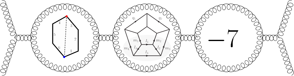
We call this fellow $\Omega$ . It’s a family of diagrams that we can write down for any number of loops: to get more loops, just extend the “…”, adding more boxes in the middle. Count the number of lines sticking out, and you get six: these are “hexagon functions”, the type of function I’ve used to calculate six-particle scattering in N=4 super Yang-Mills.

The fun thing about $\Omega$ is that we don’t have to think about it this way, one loop at a time. We can add up all the loops, $\alpha$ times one loop plus $\alpha^2$ times two loops plus $\alpha^3$ times three loops, all the way up to infinity. And we’ve managed to figure out what those loops sum to.

omegaeqnpic

The result ends up beautifully simple. This formula isn’t just true for small coupling constants, it’s true for any number you care to plug in, making the forces as strong as you’d like.

We can do this with $\Omega$ because we have equations relating different loops together. Solving those equations with a few educated guesses, we can figure out the full sum. We can also go back, and use those equations to take the $\Omega$ s at each loop apart, finding a basis of functions needed to describe them.

That basis is the real reward here. It’s not the full basis of “hexagon functions”: if you wanted to do a full six-particle calculation, you’d need more functions than the ones $\Omega$ is made of. What it is, though, is a basis we can describe completely, stating exactly what it’s made of for any number of loops.

We can’t do that with the hexagon functions, at least not yet: we have to build them loop by loop, one at a time before we can find the next ones. The hope, though, is that we won’t have to do this much longer. The $\Omega$ basis covers some of the functions we need. Our hope is that other nice families of diagrams can cover the rest. If we can identify more functions like $\Omega$ , things that we can sum to any number of loops, then perhaps we won’t have to think loop by loop anymore. If we know the right building blocks, we might be able to guess the whole amplitude, to find a formula that works for any $\alpha$ you’d like.

That would be a big deal. N=4 super Yang-Mills isn’t the real world, but it’s complicated in some of the same ways. If we can calculate there without approximations, it should at least give us an idea of what part of the real-world answer can look like. And for a field that almost always uses approximations, that’s some pretty substantial progress.

Calabi-Yaus for Higgs Phenomenology

8 Replies

less joking title:

You Didn’t Think We’d Stop at Elliptics, Did You?

When calculating scattering amplitudes, I like to work with polylogarithms. They’re a very well-understood type of mathematical function, and thus pretty easy to work with.

Even for our favorite theory of N=4 super Yang-Mills, though, they’re not the whole story. You need other types of functions to represent amplitudes, elliptic polylogarithms that are only just beginning to be properly understood. We had our own modest contribution to that topic last year.

You can think of the difference between these functions in terms of more and more complicated curves. Polylogarithms just need circles or spheres, elliptic polylogarithms can be described with a torus.

A torus is far from the most complicated curve you can think of, though.

String theorists have done a lot of research into complicated curves, in particular ones with a property called Calabi-Yau. They were looking for ways to curl up six or seven extra dimensions, to get down to the four we experience. They wanted to find ways of curling that preserved some supersymmetry, in the hope that they could use it to predict new particles, and it turned out that Calabi-Yau was the condition they needed.

That hope, for the most part, didn’t pan out. There were too many Calabi-Yaus to check, and the LHC hasn’t seen any supersymmetric particles. Today, “string phenomenologists”, who try to use string theory to predict new particles, are a relatively small branch of the field.

This research did, however, have lasting impact: due to string theorists’ interest, there are huge databases of Calabi-Yau curves, and fruitful dialogues with mathematicians about classifying them.

This has proven quite convenient for us, as we happen to have some Calabi-Yaus to classify.

Our midnight train going anywhere…in the space of Calabi-Yaus

We call Feynman diagrams like the one above “traintrack integrals”. With two loops, it’s the elliptic integral we calculated last year. With three, though, you need a type of Calabi-Yau curve called a K3. With four loops, it looks like you start needing Calabi-Yau three-folds, the type of space used to compactify string theory to four dimensions.

“We” in this case is myself, Jacob Bourjaily, Andrew McLeod, Matthias Wilhelm, and Yang-Hui He, a Calabi-Yau expert we brought on to help us classify these things. Our new paper investigates these integrals, and the more and more complicated curves needed to compute them.

Calabi-Yaus had been seen in amplitudes before, in diagrams called “sunrise” or “banana” integrals. Our example shows that they should occur much more broadly. “Traintrack” integrals appear in our favorite N=4 super Yang-Mills theory, but they also appear in theories involving just scalar fields, like the Higgs boson. For enough loops and particles, we’re going to need more and more complicated functions, not just the polylogarithms and elliptic polylogarithms that people understand.

(And to be clear, no, nobody needs to do this calculation for Higgs bosons in practice. This diagram would calculate the result of two Higgs bosons colliding and producing ten or more Higgs bosons, all at energies so high you can ignore their mass, which is…not exactly relevant for current collider phenomenology. Still, the title proved too tempting to resist.)

Is there a way to understand traintrack integrals like we understand polylogarithms? What kinds of Calabi-Yaus do they pick out, in the vast space of these curves? We’d love to find out. For the moment, we just wanted to remind all the people excited about elliptic polylogarithms that there’s quite a bit more strangeness to find, even if we don’t leave the tracks.

The Amplitudes Long View

3 Replies

Occasionally, other physicists ask me what the goal of amplitudes research is. What’s it all about?

I want to give my usual answer: we’re calculating scattering amplitudes! We’re trying to compute them more efficiently, taking advantage of simplifications and using a big toolbox of different approaches, and…

Usually by this point in the conversation, it’s clear that this isn’t what they were asking.

When physicists ask me about the goal of amplitudes research, they’ve got a longer view in mind. Maybe they’ve seen a talk by Nima Arkani-Hamed, declaring that spacetime is doomed. Maybe they’ve seen papers arguing that everything we know about quantum field theory can be derived from a few simple rules. Maybe they’ve heard slogans, like “on-shell good, off-shell bad”. Maybe they’ve heard about the conjecture that N=8 supergravity is finite, or maybe they’ve just heard someone praise the field as “demoting the sacred cows like fields, Lagrangians, and gauge symmetry”.

Often, they’ve heard a little bit of all of these. Sometimes they’re excited, sometimes they’re skeptical, but either way, they’re usually more than a little confused. They’re asking how all of these statements fit into a larger story.

The glib answer is that they don’t. Amplitudes has always been a grab-bag of methods: different people with different backgrounds, united by their interest in a particular kind of calculation.

With that said, I think there is a shared philosophy, even if each of us approaches it a little differently. There is an overall principle that unites the amplituhedron and color-kinematics duality, the CHY string and bootstrap methods, BCFW and generalized unitarity.

If I had to describe that principle in one word, I’d call it minimality. Quantum field theory involves hugely complicated mathematical machinery: Lagrangians and path integrals, Feynman diagrams and gauge fixing. At the end of the day, if you want to answer a concrete question, you’re computing a few specific kinds of things: mostly, scattering amplitudes and correlation functions. Amplitudes tries to start from the other end, and ask what outputs of this process are allowed. The idea is to search for something minimal: a few principles that, when applied to a final answer in a particular form, specify it uniquely. The form in question varies: it can be a geometric picture like the amplituhedron, or a string-like worldsheet, or a constructive approach built up from three-particle amplitudes. The goal, in each case, is the same: to skip the usual machinery, and understand the allowed form for the answer.

From this principle, where do the slogans come from? How could minimality replace spacetime, or solve quantum gravity?

It can’t…if we stick to only matching quantum field theory. As long as each calculation matches one someone else could do with known theories, even if we’re more efficient, these minimal descriptions won’t really solve these kinds of big-picture mysteries.

The hope (and for the most part, it’s a long-term hope) is that we can go beyond that. By exploring minimal descriptions, the hope is that we will find not only known theories, but unknown ones as well, theories that weren’t expected in the old understanding of quantum field theory. The amplituhedron doesn’t need space-time, it might lead the way to a theory that doesn’t have space-time. If N=8 supergravity is finite, it could suggest new theories that are finite. The story repeats, with variations, whenever amplitudeologists explore the outlook of our field. If we know the minimal requirements for an amplitude, we could find amplitudes that nobody expected.

I’m not claiming we’re the only field like this: I feel like the conformal bootstrap could tell a similar story. And I’m not saying everyone thinks about our field this way: there’s a lot of deep mathematics in just calculating amplitudes, and it fascinated people long before the field caught on with the Princeton set.

But if you’re asking what the story is for amplitudes, the weird buzz you catch bits and pieces of and can’t quite put together…well, if there’s any unifying story, I think it’s this one.

4 gravitons

Stories about physics from someone who's been there