Category Archives: Amplitudes Methods

At Amplitudes 2023 at CERN

I’m at the big yearly conference of my sub-field this week, called Amplitudes. This year, surprisingly for the first time, it’s at the very appropriate location of CERN.

Somewhat overshadowed by the very picturesque Alps

Amplitudes keeps on growing. In 2019, we had 175 participants. We were on Zoom in 2020 and 2021, with many more participants, but that probably shouldn’t count. In Prague last year we had 222. This year, I’ve been told we have even more, something like 250 participants (the list online is bigger, but includes people joining on Zoom). We’ve grown due to new students, but also new collaborations: people from adjacent fields who find the work interesting enough to join along. This year we have mathematicians talking about D-modules, bootstrappers finding new ways to get at amplitudes in string theory, beyond-the-standard-model theorists talking about effective field theories, and cosmologists talking about the large-scale structure of the universe.

The talks have been great, from clear discussions of earlier results to fresh-off-the-presses developments, plenty of work in progress, and even one talk where the speaker’s opinion changed during the coffee break. As we’re at CERN, there’s also a through-line about the future of particle physics, with a chat between Nima Arkani-Hamed and the experimentalist Beate Heinemann on Tuesday and a talk by Michelangelo Mangano about the meaning of “new physics” on Thursday.

I haven’t had a ton of time to write, I keep getting distracted by good discussions! As such, I’ll do my usual thing, and say a bit more about specific talks in next week’s post.

Cabinet of Curiosities: The Deluxe Train Set

I’ve got a new paper out this week with Andrew McLeod. I’m thinking of it as another entry in this year’s “cabinet of curiosities”, interesting Feynman diagrams with unusual properties. Although this one might be hard to fit into a cabinet.

Over the past few years, I’ve been finding Feynman diagrams with interesting connections to Calabi-Yau manifolds, the spaces originally studied by string theorists to roll up their extra dimensions. With Andrew and other collaborators, I found an interesting family of these diagrams called traintracks, which involve higher-and-higher dimensional manifolds as they get longer and longer.

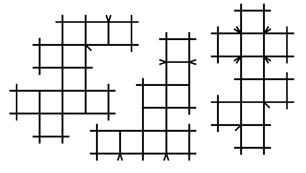
This time, we started hooking up our traintracks together.

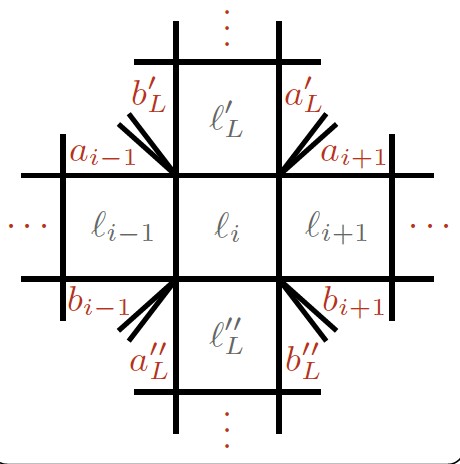
We call diagrams like these traintrack network diagrams, or traintrack networks for short. The original traintracks just went “one way”: one family, going higher in Calabi-Yau dimension the longer they got. These networks branch out, one traintrack leading to another and another.

In principle, these are much more complicated diagrams. But we find we can work with them in almost the same way. We can find the same “starting point” we had for the original traintracks, the set of integrals used to find the Calabi-Yau manifold. We’ve even got more reliable tricks, a method recently honed by some friends of ours that consistently find a Calabi-Yau manifold inside the original traintracks.

Surprisingly, though, this isn’t enough.

It works for one type of traintrack network, a so-called “cross diagram” like this:

But for other diagrams, if the network branches any more, the trick stops working. We still get an answer, but that answer is some more general space, not just a Calabi-Yau manifold.

That doesn’t mean that these general traintrack networks don’t involve Calabi-Yaus at all, mind you: it just means this method doesn’t tell us one way or the other. It’s also possible that simpler versions of these diagrams, involving fewer particles, will once again involve Calabi-Yaus. This is the case for some similar diagrams in two dimensions. But it’s starting to raise a question: how special are the Calabi-Yau related diagrams? How general do we expect them to be?

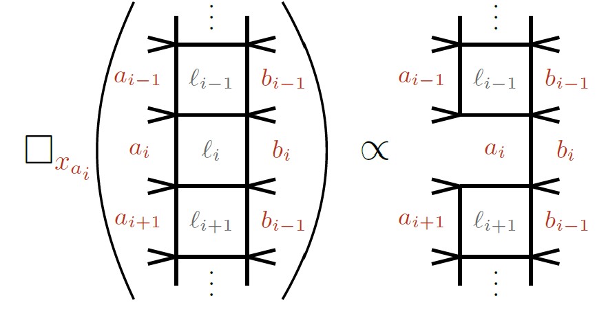
Another fun thing we noticed has to do with differential equations. There are equations that relate one diagram to another simpler one. We’ve used them in the past to build up “ladders” of diagrams, relating each picture to one with one of its boxes “deleted”. We noticed, playing with these traintrack networks, that these equations do a bit more than we thought. “Deleting” a box can make a traintrack short, but it can also chop a traintrack in half, leaving two “dangling” pieces, one on either side.

This reminded me of an important point, one we occasionally lose track of. The best-studied diagrams related to Calabi-Yaus are called “sunrise” diagrams. If you squish together a loop in one of those diagrams, the whole diagram squishes together, becoming much simpler. Because of that, we’re used to thinking of these as diagrams with a single “geometry”, one that shows up when you don’t “squish” anything.

Traintracks, and traintrack networks, are different. “Squishing” the diagram, or “deleting” a box, gives you a simpler diagram, but not much simpler. In particular, the new diagram will still contain traintracks, and traintrack networks. That means that we really should think of each traintrack network not just as one “top geometry”, but of a collection of geometries, different Calabi-Yaus that break into different combinations of Calabi-Yaus in different ways. It’s something we probably should have anticipated, but the form these networks take is a good reminder, one that points out that we still have a lot to do if we want to understand these diagrams.

Cabinet of Curiosities: The Train-Ladder

I’ve got a new paper out this week, with Andrew McLeod, Roger Morales, Matthias Wilhelm, and Chi Zhang. It’s yet another entry in this year’s “cabinet of curiosities”, quirky Feynman diagrams with interesting traits.

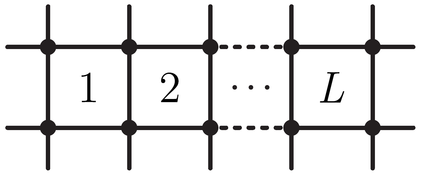
A while back, I talked about a set of Feynman diagrams I could compute with any number of “loops”, bypassing the approximations we usually need to use in particle physics. That wasn’t the first time someone did that. Back in the 90’s, some folks figured out how to do this for so-called “ladder” diagrams. These diagrams have two legs on one end for two particles coming in, two legs on the other end for two particles going out, and a ladder in between, like so:

There are infinitely many of these diagrams, but they’re all beautifully simple, variations on a theme that can be written down in a precise mathematical way.

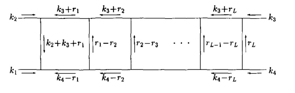
Change things a little bit, though, and the situation gets wildly more intractable. Let the rungs of the ladder peek through the sides, and you get something looking more like the tracks for a train:

These traintrack integrals are much more complicated. Describing them requires the mathematics of Calabi-Yau manifolds, involving higher and higher dimensions as the tracks get longer. I don’t think there’s any hope of understanding these things for all loops, at least not any time soon.

What if we aimed somewhere in between? A ladder that just started to turn traintrack?

Add just a single pair of rungs, and it turns out that things remain relatively simple. If we do this, it turns out we don’t need any complicated Calabi-Yau manifolds. We just need the simplest Calabi-Yau manifold, called an elliptic curve. It’s actually the same curve for every version of the diagram. And the situation is simple enough that, with some extra cleverness, it looks like we’ve found a trick to calculate these diagrams to any number of loops we’d like.

(Another group figured out the curve, but not the calculation trick. They’ve solved different problems, though, studying all sorts of different traintrack diagrams. They sorted out some confusion I used to have about one of those diagrams, showing it actually behaves precisely the way we expected it to. All in all, it’s been a fun example of the way different scientists sometimes hone in on the same discovery.)

These developments are exciting, because Feynman diagrams with elliptic curves are still tough to deal with. We still have whole conferences about them. These new elliptic diagrams can be a long list of test cases, things we can experiment with with any number of loops. With time, we might truly understand them as well as the ladder diagrams!

This Week at Quanta Magazine

I’ve got an article in Quanta Magazine this week, about a program called FORM.

Quanta has come up a number of times on this blog, they’re a science news outlet set up by the Simons Foundation. Their goal is to enhance the public understanding of science and mathematics. They cover topics other outlets might find too challenging, and they cover the topics others cover with more depth. Most people I know who’ve worked with them have been impressed by their thoroughness: they take fact-checking to a level I haven’t seen with other science journalists. If you’re doing a certain kind of mathematical work, then you hope that Quanta decides to cover it.

A while back, as I was chatting with one of their journalists, I had a startling realization: if I want Quanta to cover something, I can send them a tip, and if they’re interested they’ll write about it. That realization resulted in the article I talked about here. Chatting with the journalist interviewing me for that article, though, I learned something if anything even more startling: if I want Quanta to cover something, and I want to write about it, I can pitch the article to Quanta, and if they’re interested they’ll pay me to write about it.

Around the same time, I happened to talk to a few people in my field, who had a problem they thought Quanta should cover. A software, called FORM, was used in all the most serious collider physics calculations. Despite that, the software wasn’t being supported: its future was unclear. You can read the article to learn more.

One thing I didn’t mention in that article: I hadn’t used FORM before I started writing it. I don’t do those “most serious collider physics calculations”, so I’d never bothered to learn FORM. I mostly use Mathematica, a common choice among physicists who want something easy to learn, even if it’s not the strongest option for many things.

(By the way, it was surprisingly hard to find quotes about FORM that didn’t compare it specifically to Mathematica. In the end I think I included one, but believe me, there could have been a lot more.)

Now, I wonder if I should have been using FORM all along. Many times I’ve pushed to the limits of what Mathematica could comfortable handle, the limits of what my computer’s memory could hold, equations long enough that just expanding them out took complicated work-arounds. If I had learned FORM, maybe I would have breezed through those calculations, and pushed even further.

I’d love it if this article gets FORM more attention, and more support. But also, I’d love it if it gives a window on the nuts and bolts of hard-core particle physics: the things people have to do to turn those T-shirt equations into predictions for actual colliders. It’s a world in between physics and computer science and mathematics, a big part of the infrastructure of how we know what we know that, precisely because it’s infrastructure, often ends up falling through the cracks.

Edit: For researchers interested in learning more about FORM, the workshop I mentioned at the end of the article is now online, with registrations open.

Jumpstarting Elliptic Bootstrapping

I was at a mini-conference this week, called Jumpstarting Elliptic Bootstrap Methods for Scattering Amplitudes.

I’ve done a lot of work with what we like to call “bootstrap” methods. Instead of doing a particle physics calculation in all its gory detail, we start with a plausible guess and impose requirements based on what we know. Eventually, we have the right answer pulled up “by its own bootstraps”: the only answer the calculation could have, without actually doing the calculation.

This method works very well, but so far it’s only been applied to certain kinds of calculations, involving mathematical functions called polylogarithms. More complicated calculations involve a mathematical object called an elliptic curve, and until very recently it wasn’t clear how to bootstrap them. To get people thinking about it, my colleagues Hjalte Frellesvig and Andrew McLeod asked the Carlsberg Foundation (yes, that Carlsberg) to fund a mini-conference. The idea was to get elliptic people and bootstrap people together (along with Hjalte’s tribe, intersection theory people) to hash things out. “Jumpstart people” are not a thing in physics, so despite the title they were not invited.

Anyone remember these games? Did you know that they still exist, have an educational MMO, and bought neopets?

Having the conference so soon after the yearly Elliptics meeting had some strange consequences. There was only one actual duplicate talk, but the first day of talks all felt like they would have been welcome additions to the earlier conference. Some might be functioning as “overflow”: Elliptics this year focused on discussion and so didn’t have many slots for talks, while this conference despite its discussion-focused goal had a more packed schedule. In other cases, people might have been persuaded by the more relaxed atmosphere and lack of recording or posted slides to give more speculative talks. Oliver Schlotterer’s talk was likely in this category, a discussion of the genus-two functions one step beyond elliptics that I think people at the previous conference would have found very exciting, but which involved work in progress that I could understand him being cautious about presenting.

The other days focused more on the bootstrap side, with progress on some surprising but not-quite-yet elliptic avenues. It was great to hear that Mark Spradlin is making new progress on his Ziggurat story, to hear James Drummond suggest a picture for cluster algebras that could generalize to other theories, and to get some idea of the mysterious ongoing story that animates my colleague Cristian Vergu.

There was one thing the organizers couldn’t have anticipated that ended up throwing the conference into a new light. The goal of the conference was to get people started bootstrapping elliptic functions, but in the meantime people have gotten started on their own. Roger Morales Espasa presented his work on this with several of my other colleagues. They can already reproduce a known result, the ten-particle elliptic double-box, and are well on-track to deriving something genuinely new, the twelve-particle version. It’s exciting, but it definitely makes the rest of us look around and take stock. Hopefully for the better!

Cabinet of Curiosities: The Nested Toy

I had a paper two weeks ago with a Master’s student, Alex Chaparro Pozo. I haven’t gotten a chance to talk about it yet, so I thought I should say a few words this week. It’s another entry in what I’ve been calling my cabinet of curiosities, interesting mathematical “objects” I’m sharing with the world.

I calculate scattering amplitudes, formulas that give the probability that particles scatter off each other in particular ways. While in principle I could do this with any particle physics theory, I have a favorite: a “toy model” called N=4 super Yang-Mills. N=4 super Yang-Mills doesn’t describe reality, but it lets us figure out cool new calculation tricks, and these often end up useful in reality as well.

Many scattering amplitudes in N=4 super Yang-Mills involve a type of mathematical functions called polylogarithms. These functions are especially easy to work with, but they aren’t the whole story. One we start considering more complicated situations (what if two particles collide, and eight particles come out?) we need more complicated functions, called elliptic polylogarithms.

A few years ago, some collaborators and I figured out how to calculate one of these elliptic scattering amplitudes. We didn’t do it as well as we’d like, though: the calculation was “half-done” in a sense. To do the other half, we needed new mathematical tools, tools that came out soon after. Once those tools were out, we started learning how to apply them, trying to “finish” the calculation we started.

The original calculation was pretty complicated. Two particles colliding, eight particles coming out, meant that in total we had to keep track of ten different particles. That gets messy fast. I’m pretty good at dealing with six particles, not ten. Luckily, it turned out there was a way to pretend there were six particles only: by “twisting” up the calculation, we found a toy model within the toy model: a six-particle version of the calculation. Much like the original was in a theory that doesn’t describe the real world, these six particles don’t describe six particles in that theory: they’re a kind of toy calculation within the toy model, doubly un-real.

Not quintuply-unreal though

With this nested toy model, I was confident we could do the calculation. I wasn’t confident I’d have time for it, though. This ended up making it perfect for a Master’s thesis, which is how Alex got into the game.

Alex worked his way through the calculation, programming and transforming, going from one type of mathematical functions to another (at least once because I’d forgotten to tell him the right functions to use, oops!) There were more details and subtleties than expected, but in the end everything worked out.

Then, we were scooped.

Another group figured out how to do the full, ten-particle problem, not just the toy model. That group was just “down the hall”…or would have been “down the hall” if we had been going to the office (this was 2021, after all). I didn’t hear about what they were working on until it was too late to change plans.

Alex left the field (not, as far as I know, because of this). And for a while, because of that especially thorough scooping, I didn’t publish.

What changed my mind, in part, was seeing the field develop in the meantime. It turns out toy models, and even nested toy models, are quite useful. We still have a lot of uncertainty about what to do, how to use the new calculation methods and what they imply. And usually, the best way to get through that kind of uncertainty is with simple, well-behaved toy models.

So I thought, in the end, that this might be useful. Even if it’s a toy version of something that already exists, I expect it to be an educational toy, one we can learn a lot from. So I’ve put it out into the world, as part of this year’s cabinet of curiosities.

At Elliptic Integrals in Fundamental Physics in Mainz

I’m at a conference this week. It’s named Elliptic Integrals in Fundamental Physics, but I think of it as “Elliptics 2022”, the latest in a series of conferences on elliptic integrals in particle physics.

It’s in Mainz, which you can tell from the Gutenberg street art

Elliptics has been growing in recent years, hurtling into prominence as a subfield of amplitudes (which is already a subfield of theoretical physics). This has led to growing lists of participants and a more and more packed schedule.

This year walked all of that back a bit. There were three talks a day: two one-hour talks by senior researchers and one half-hour talk by a junior researcher. The rest, as well as the whole last day, are geared to discussion. It’s an attempt to go back to the subfield’s roots. In the beginning, the Elliptics conferences drew together a small group to sort out a plan for the future, digging through the often-confusing mathematics to try to find a baseline for future progress. The field has advanced since then, but some of our questions are still almost as basic. What relations exist between different calculations? How much do we value fast numerics, versus analytical understanding? What methods do we want to preserve, and which aren’t serving us well? To answer these questions, it helps to get a few people together in one place, not to silently listen to lectures, but to question and discuss and hash things out. I may have heard a smaller range of topics at this year’s Elliptics, but due to the sheer depth we managed to probe on those fewer topics I feel like I’ve learned much more.

Since someone always asks, I should say that the talks were not recorded, but they are posting slides online, so if you’re interested in the topic you can watch there. A few people discussed new developments, some just published and some yet to be published. I discussed the work I talked about last week, and got a lot of good feedback and ideas about how to move forward.

Cabinet of Curiosities: The Coaction

I had two more papers out this week, continuing my cabinet of curiosities. I’ll talk about one of them today, and the other in (probably) two weeks.

This week, I’m talking about a paper I wrote with an excellent Master’s student, Andreas Forum. Andreas came to me looking for a project on the mathematical side. I had a rather nice idea for his project at first, to explain a proof in an old math paper so it could be used by physicists.

Unfortunately, the proof I sent him off to explain didn’t actually exist. Fortunately, by the time we figured this out Andreas had learned quite a bit of math, so he was ready for his next project: a coaction for Calabi-Yau Feynman diagrams.

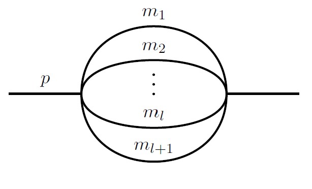
We chose to focus on one particular diagram, called a sunrise diagram for its resemblance to a sun rising over the sea:

This diagram

Feynman diagrams depict paths traveled by particles. The paths are a metaphor, or organizing tool, for more complicated calculations: computations of the chances fundamental particles behave in different ways. Each diagram encodes a complicated integral. This one shows one particle splitting into many, then those many particles reuniting into one.

Do the integrals in Feynman diagrams, and you get a variety of different mathematical functions. Many of them integrate to functions called polylogarithms, and we’ve gotten really really good at working with them. We can integrate them up, simplify them, and sometimes we can guess them so well we don’t have to do the integrals at all! We can do all of that because we know how to break polylogarithm functions apart, with a mathematical operation called a coaction. The coaction chops polylogarithms up to simpler parts, parts that are easier to work with.

More complicated Feynman diagrams give more complicated functions, though. Some of them give what are called elliptic functions. You can think of these functions as involving a geometrical shape, in this case a torus.

Other functions involve more complicated geometrical shapes, in some cases very complicated. For example, some involve the Calabi-Yau manifolds studied by string theorists. These sunrise diagrams are some of the simplest to involve such complicated geometry.

Other researchers had proposed a coaction for elliptic functions back in 2018. When they derived it, though, they left a recipe for something more general. Follow the instructions in the paper, and you could in principle find a coaction for other diagrams, even the Calabi-Yau ones, if you set it up right.

I had an idea for how to set it up right, and in the grand tradition of supervisors everywhere I got Andreas to do the dirty work of applying it. Despite the delay of our false start and despite the fact that this was probably in retrospect too big a project for a normal Master’s thesis, Andreas made it work!

Our result, though, is a bit weird. The coaction is a powerful tool for polylogarithms because it chops them up finely: keep chopping, and you get down to very simple functions. Our coaction isn’t quite so fine: we don’t chop our functions into as many parts, and the parts are more mysterious, more difficult to handle.

We think these are temporary problems though. The recipe we applied turns out to be a recipe with a lot of choices to make, less like Julia Child and more like one of those books where you mix-and-match recipes. We believe the community can play with the parameters of this recipe, finding new version of the coaction for new uses.

This is one of the shiniest of the curiosities in my cabinet this year, I hope it gets put to good use.

Cabinet of Curiosities: The Cubic

Before I launch into the post: I got interviewed on Theoretically Podcasting, a new YouTube channel focused on beginning grad student-level explanations of topics in theoretical physics. If that sounds interesting to you, check it out!

This Fall is paper season for me. I’m finishing up a number of different projects, on a number of different things. Each one was its own puzzle: a curious object found, polished, and sent off into the world.

Monday I published the first of these curiosities, along with Jake Bourjaily and Cristian Vergu.

I’ve mentioned before that the calculations I do involve a kind of “alphabet“. Break down a formula for the probability that two particles collide, and you find pieces that occur again and again. In the nicest cases, those pieces are rational functions, but they can easily get more complicated. I’ve talked before about a case where square roots enter the game, for example. But if square roots appear, what about something even more complicated? What about cubic roots?

What about 1024th roots?

Occasionally, my co-authors and I would say something like that at the end of a talk and an older professor would scoff: “Cube roots? Impossible!”

You might imagine these professors were just being unreasonable skeptics, the elderly-but-distinguished scientists from that Arthur C. Clarke quote. But while they turned out to be wrong, they weren’t being unreasonable. They were thinking back to theorems from the 60’s, theorems which seemed to argue that these particle physics calculations could only have a few specific kinds of behavior: they could behave like rational functions, like logarithms, or like square roots. Theorems which, as they understood them, would have made our claims impossible.

Eventually, we decided to figure out what the heck was going on here. We grabbed the simplest example we could find (a cube root involving three loops and eleven gluons in N=4 super Yang-Mills…yeah) and buckled down to do the calculation.

When we want to calculate something specific to our field, we can reference textbooks and papers, and draw on our own experience. Much of the calculation was like that. A crucial piece, though, involved something quite a bit less specific: calculating a cubic root. And for things like that, you can tell your teachers we use only the very best: Wikipedia.

Check out the Wikipedia entry for the cubic formula. It’s complicated, in ways the quadratic formula isn’t. It involves complex numbers, for one. But it’s not that crazy.

What those theorems from the 60’s said (and what they actually said, not what people misremembered them as saying), was that you can’t take a single limit of a particle physics calculation, and have it behave like a cubic root. You need to take more limits, not just one, to see it.

It turns out, you can even see this just from the Wikipedia entry. There’s a big cube root sign in the middle there, equal to some variable “C”. Look at what’s inside that cube root. You want that part inside to vanish. That means two things need to cancel: Wikipedia labels them \Delta_1, and \sqrt{\Delta_1^2-4\Delta_0^3}. Do some algebra, and you’ll see that for those to cancel, you need \Delta_0=0.

So you look at the limit, \Delta_0\rightarrow 0. This time you need not just some algebra, but some calculus. I’ll let the students in the audience work it out, but at the end of the day, you should notice how C behaves when \Delta_0 is small. It isn’t like \sqrt[3]{\Delta_0}. It’s like just plain \Delta_0. The cube root goes away.

It can come back, but only if you take another limit: not just \Delta_0\rightarrow 0, but \Delta_1\rightarrow 0 as well. And that’s just fine according to those theorems from the 60’s. So our cubic curiosity isn’t impossible after all.

Our calculation wasn’t quite this simple, of course. We had to close a few loopholes, checking our example in detail using more than just Wikipedia-based methods. We found what we thought was a toy example, that turned out to be even more complicated, involving roots of a degree-six polynomial (one that has no “formula”!).

And in the end, polished and in their display case, we’ve put our examples up for the world to see. Let’s see what people think of them!

Why the Antipode Was Supposed to Be Useless

A few weeks back, Quanta Magazine had an article about a new discovery in my field, called antipodal duality.

Some background: I’m a theoretical physicist, and I work on finding better ways to make predictions in particle physics. Folks in my field make these predictions with formulas called “scattering amplitudes” that encode the probability that particles bounce, or scatter, in particular ways. One trick we’ve found is that these formulas can often be written as “words” in a kind of “alphabet”. If we know the alphabet, we can make our formulas much simpler, or even guess formulas we could never have calculated any other way.

Quanta’s article describes how a few friends of mine (Lance Dixon, Ömer Gürdoğan, Andrew McLeod, and Matthias Wilhelm) noticed a weird pattern in two of these formulas, from two different calculations. If you flip the “words” around, back to front (an operation called the antipode), you go from a formula describing one collision of particles to a formula for totally different particles. Somehow, the two calculations are “dual”: two different-seeming descriptions that secretly mean the same thing.

Quanta quoted me for their article, and I was (pleasantly) baffled. See, the antipode was supposed to be useless. The mathematicians told us it was something the math allows us to do, like you’re allowed to order pineapple on pizza. But just like pineapple on pizza, we couldn’t imagine a situation where we actually wanted to do it.

What Quanta didn’t say was why we thought the antipode was useless. That’s a hard story to tell, one that wouldn’t fit in a piece like that.

It fits here, though. So in the rest of this post, I’d like to explain why flipping around words is such a strange, seemingly useless thing to do. It’s strange because it swaps two things that in physics we thought should be independent: branch cuts and derivatives, or particles and symmetries.

Let’s start with the first things in each pair: branch cuts, and particles.

The first few letters of our “word” tell us something mathematical, and they tell us something physical. Mathematically, they tell us ways that our formula can change suddenly, and discontinuously.

Take a logarithm, the inverse of e^x. You’re probably used to plugging in positive numbers, and getting out something reasonable, that changes in a smooth and regular way: after all, e^x is always positive, right? But in mathematics, you don’t have to just use positive numbers. You can use negative numbers. Even more interestingly, you can use complex numbers. And if you take the logarithm of a complex number, and look at the imaginary part, it looks like this:

Mostly, this complex logarithm still seems to be doing what it’s supposed to, changing in a nice slow way. But there is a weird “cut” in the graph for negative numbers: a sudden jump, from \pi to -\pi. That jump is called a “branch cut”.

As physicists, we usually don’t like our formulas to make sudden changes. A change like this is an infinitely fast jump, and we don’t like infinities much either. But we do have one good use for a formula like this, because sometimes our formulas do change suddenly: when we have enough energy to make a new particle.

Imagine colliding two protons together, like at the LHC. Colliding particles doesn’t just break the protons into pieces: due to Einstein’s famous E=mc^2, it can create new particles as well. But to create a new particle, you need enough energy: mc^2 worth of energy. So as you dial up the energy of your protons, you’ll notice a sudden change: you couldn’t create, say, a Higgs boson, and now you can. Our formulas represent some of those kinds of sudden changes with branch cuts.

So the beginning of our “words” represent branch cuts, and particles. The end represents derivatives and symmetries.

Derivatives come from the land of calculus, a place spooky to those with traumatic math class memories. Derivatives shouldn’t be so spooky though. They’re just ways we measure change. If we have a formula that is smoothly changing as we change some input, we can describe that change with a derivative.

The ending of our “words” tell us what happens when we take a derivative. They tell us which ways our formulas can smoothly change, and what happens when they do.

In doing so, they tell us about something some physicists make sound spooky, called symmetries. Symmetries are changes we can make that don’t really change what’s important. For example, you could imagine lifting up the entire Large Hadron Collider and (carefully!) carrying it across the ocean, from France to the US. We’d expect that, once all the scared scientists return and turn it back on, it would start getting exactly the same results. Physics has “translation symmetry”: you can move, or “translate” an experiment, and the important stuff stays the same.

These symmetries are closely connected to derivatives. If changing something doesn’t change anything important, that should be reflected in our formulas: they shouldn’t change either, so their derivatives should be zero. If instead the symmetry isn’t quite true, if it’s what we call “broken”, then by knowing how it was “broken” we know what the derivative should be.

So branch cuts tell us about particles, derivatives tell us about symmetries. The weird thing about the antipode, the un-physical bizarre thing, is that it swaps them. It makes the particles of one calculation determine the symmetries of another.

(And lest you’ve heard about particles with symmetries, like gluons and SU(3)…this is a different kind of thing. I don’t have enough room to explain why here, but it’s completely unrelated.)

Why the heck does this duality exist?

A commenter on the last post asked me to speculate. I said there that I have no clue, and that’s most of the answer.

If I had to speculate, though, my answer might be disappointing.

Most of the things in physics we call “dualities” have fairly deep physical meanings, linked to twisting spacetime in complicated ways. AdS/CFT isn’t fully explained, but it seems to be related to something called the holographic principle, the idea that gravity ties together the inside of space with the boundary around it. T duality, an older concept in string theory, is explained: a consequence of how strings “see” the world in terms of things to wrap around and things to spin around. In my field, one of our favorite dualities links back to this as well, amplitude-Wilson loop duality linked to fermionic T-duality.

The antipode doesn’t twist spacetime, it twists the mathematics. And it may be it matters only because the mathematics is so constrained that it’s forced to happen.

The trick that Lance Dixon and co. used to discover antipodal duality is the same trick I used with Lance to calculate complicated scattering amplitudes. It relies on taking a general guess of words in the right “alphabet”, and constraining it: using mathematical and physical principles it must obey and throwing out every illegal answer until there’s only one answer left.

Currently, there are some hints that the principles used for the different calculations linked by antipodal duality are “antipodal mirrors” of each other: that different principles have the same implication when the duality “flips” them around. If so, then it could be this duality is in some sense just a coincidence: not a coincidence limited to a few calculations, but a coincidence limited to a few principles. Thought of in this way, it might not tell us a lot about other situations, it might not really be “deep”.

Of course, I could be wrong about this. It could be much more general, could mean much more. But in that context, I really have no clue what to speculate. The antipode is weird: it links things that really should not be physically linked. We’ll have to see what that actually means.