Tag Archives: string theory

Does Science have Fads?

97% of climate scientists agree that global warming exists, and is most probably human-caused. On a more controversial note, string theorists vastly outnumber adherents of other approaches to quantum gravity, such as Loop Quantum Gravity.

As many who disagree with climate change or string theory would argue, the majority is not always right. Science should be concerned with truth, not merely with popularity. After all, what if scientists are merely taking part in a fad? What makes climate change any more objectively true than pet rocks?

Apparently this wikipedia’s best example of a fad.

People are susceptible to fads, after all. A style of music becomes popular, and everyone’s listening to the same sounds. A style of clothing, and everything’s wearing the same thing. So if an idea in science became popular, everyone might…write the same papers?

That right there is the problem. Scientists only succeed by creating meaningfully original work. If we don’t discover something new, we can’t publish, and as the old saying goes it’s publish or perish out there. Even if social pressure gets us working on something, if we’re going to get any actual work done there has to be enough there, at least, for us to do something different, something no-one has done before.

This doesn’t mean scientists can’t be influenced by popularity, but it means that that influence is limited by the requirements of doing meaningful, original work. In the case of climate change, climate scientists investigate the topic with so many different approaches and look at so many different areas of impact (for example, did you know rising CO2 levels make the ocean acidic?) that the whole field simply wouldn’t function if climate change wasn’t real: there’d be a contradiction, and most of the myriad projects involving it simply wouldn’t work. As I’ve talked about before, science is an interlocking system, and it’s hard to doubt one part without being forced to doubt everything else.

What about string theory? Here, the situation is a little different. There aren’t experiments testing string theory, so whether or not string theory describes the real world won’t have much effect on whether people can write string theory papers.

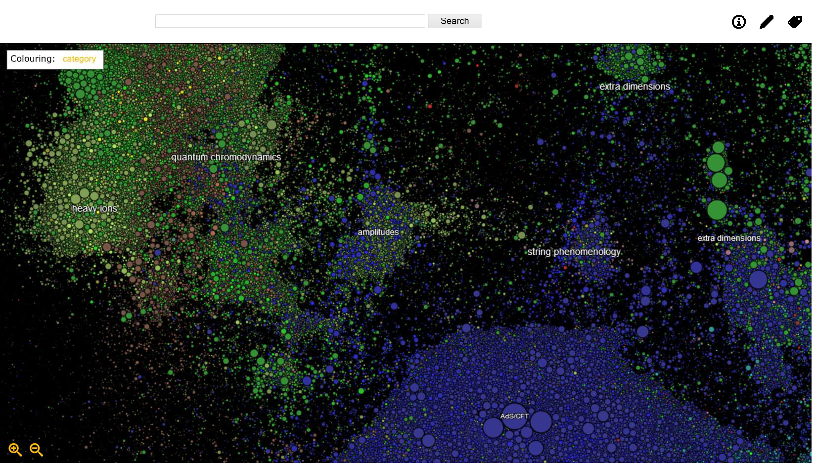
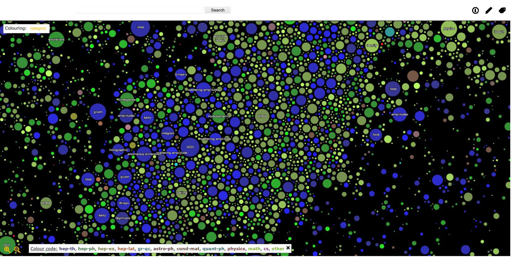
The existence of so many string theory papers does say something, though. The up-side of not involving experiments is that you can’t go and test something slightly different and write a paper about it. In order to be original, you really need to calculate something that nobody expected you to calculate, or notice a trend nobody expected to exist. The fact that there are so many more string theorists than loop quantum gravity theorists is in part because there are so many more interesting string theory projects than interesting loop quantum gravity projects.

In string theory, projects tend to be interesting because they unveil some new aspect of quantum field theory, the class of theories that explain the behavior of subatomic particles. Given how hard quantum field theory is, any insight is valuable, and in my experience these sorts of insights are what most string theorists are after. So while string theory’s popularity says little about whether it describes the real world, it says a lot about its ability to say interesting things about quantum field theory. And since quantum field theories do describe the real world, string theory’s continued popularity is also evidence that it continues to be useful.

Climate change and string theory aren’t fads, not exactly. They’re popular, not simply because they’re popular, but because they make important contributions and valuable to science. And as long as science continues to reward original work, that’s not about to change.

Gravity is Yang-Mills Squared

12 Replies

There’s a concept that I’ve wanted to present for quite some time. It’s one of the coolest accomplishments in my subfield, but I thought that explaining it would involve too much technical detail. However, the recent BICEP2 results have brought one aspect of it to the public eye, so I’ve decided that people are ready.

If you’ve been following the recent announcements by the BICEP2 telescope of their indirect observation of primordial gravitational waves, you’ve probably seen the phrases “E-mode polarization” and “B-mode polarization” thrown around. You may even have seen pictures, showing that light in the cosmic microwave background is polarized differently by quantum fluctuations in the inflaton field and by quantum fluctuations in gravity.

But why is there a difference? What’s unique about gravitational waves that makes them different from the other waves in nature?

As it turns out, the difference all boils down to one statement:

Gravity is Yang-Mills squared.

This is both a very simple claim and a very subtle one, and it comes up in many many places in physics.

Yang-Mills, for those who haven’t read my older posts, is a general category that contains most of the fundamental forces. Electromagnetism, the strong nuclear force, and the weak nuclear force are all variants of Yang-Mills forces.

Yang-Mills forces have “spin 1”. Another way to say this is that Yang-Mills forces are vector forces. If you remember vectors from math class, you might remember that a vector has a direction and a strength. This hopefully makes sense: forces point in a direction, and have a strength. You may also remember that vectors can also be described in terms of components. A vector in four space-time dimensions has four components: x, y, z, and time, like so:

$\left( \begin{array}{c} x \\ y \\ z \\ t \end{array} \right)$

Gravity has “spin 2”.

As I’ve talked about before, gravity bends space and time, which means that it modifies the way you calculate distances. In practice, that means it needs to be something that can couple two vectors together: a matrix, or more precisely, a tensor, like so:

$\left( \begin{array}{cccc} xx & xy & xz & xt\\ yx & yy & yz & yt\\ zx & zy & zz & zt\\ tx & ty & tz & tt\end{array} \right)$

So while a Yang-Mills force has four components, gravity has sixteen. Gravity is Yang-Mills squared.

(Technical note: gravity actually doesn’t use all sixteen components, because it’s traceless and symmetric. However, often when studying gravity’s quantum properties theorists often add on extra fields to “complete the square” and fill in the remaining components.)

There’s much more to the connection than that, though. For one, it appears in the kinds of waves the two types of forces can create.

In order to create an electromagnetic wave you need a dipole, a negative charge and a positive charge at opposite ends of a line, and you need that dipole to change over time.

Change over time, of course, is a property of Gifs.

Gravity doesn’t have negative and positive charges, it just has one type of charge. Thus, to create gravitational waves you need not a dipole, but a quadrupole: instead of a line between two opposite charges, you have four gravitational charges (masses) arranged in a square. This creates a “breathing” sort of motion, instead of the back-and-forth motion of electromagnetic waves.

This is your brain on gravitational waves.

This is why gravitational waves have a different shape than electromagnetic waves, and why they have a unique effect on the cosmic microwave background, allowing them to be spotted by BICEP2. Gravity, once again, is Yang-Mills squared.

But wait there’s more!

So far, I’ve shown you that gravity is the square of Yang-Mills, but not in a very literal way. Yes, there are lots of similarities, but it’s not like you can just square a calculation in Yang-Mills and get a calculation in gravity, right?

Well actually…

In quantum field theory, calculations are traditionally done using tools called Feynman diagrams, organized by how many loops the diagram contains. The simplest diagrams have no loops, and are called tree diagrams.

Fascinatingly, for tree diagrams the message of this post is as literal as it can be. Using something called the Kawai-Lewellen-Tye relations, the result of a tree diagram calculation in gravity can be found just by taking a similar calculation in Yang-Mills and squaring it.

(Interestingly enough, these relations were originally discovered using string theory, but they don’t require string theory to work. It’s yet another example of how string theory functions as a laboratory to make discoveries about quantum field theory.)

Does this hold beyond tree diagrams? As it turns out, the answer is again yes!
The calculation involved is a little more complicated, but as discovered by Zvi Bern, John Joseph Carrasco, and Henrik Johansson, if you can get your calculation in Yang-Mills into the right format then all you need to do is square the right thing at the right step to get gravity, even for diagrams with loops!

zvi-bern-350

This trick, called BCJ duality after its discoverers, has allowed calculations in quantum gravity that far outpace what would be possible without it. In N=8 supergravity, the gravity analogue of N=4 super Yang-Mills, calculations have progressed up to four loops, and have revealed tantalizing hints that the uncontrolled infinities that usually plague gravity theories are absent in N=8 supergravity, even without adding in string theory. Results like these are why BCJ duality is viewed as one of the “foundational miracles” of the field for those of us who study scattering amplitudes.

Gravity is Yang-Mills squared, in more ways than one. And because gravity is Yang-Mills squared, gravity may just be tame-able after all.

How (Not) to Sum the Natural Numbers: Zeta Function Regularization

16 Replies

$1+2+3+4+5+6+\ldots=-\frac{1}{12}$

If you follow Numberphile on YouTube or Bad Astronomy on Slate you’ve already seen this counter-intuitive sum written out. Similarly, if you follow those people or Sciencetopia’s Good Math, Bad Math, you’re aware that the way that sum was presented by Numberphile in that video was seriously flawed.

There is a real sense in which adding up all of the natural numbers (numbers 1, 2, 3…) really does give you minus twelve, despite all the reasons this should be impossible. However, there is also a real sense in which it does not, and cannot, do any such thing. To explain this, I’m going to introduce two concepts: complex analysis and regularization.

This discussion is not going to be mathematically rigorous, but it should give an authentic and accurate view of where these results come from. If you’re interested in the full mathematical details, a later discussion by Numberphile should help, and the mathematically confident should read Terence Tao’s treatment from back in 2010.

With that said, let’s talk about sums! Well, one sum in particular:

$\frac{1}{1^s}+\frac{1}{2^s}+\frac{1}{3^s}+\frac{1}{4^s}+\frac{1}{5^s}+\frac{1}{6^s}+\ldots = \zeta(s)$

If s is greater than one, then each term in this infinite sum gets smaller and smaller fast enough that you can add them all up and get a number. That number is referred to as $\zeta(s)$ , the Riemann Zeta Function.

So what if s is smaller than one?

The infinite sum that I described doesn’t converge for s less than one. Add it up in any reasonable way, and it just approaches infinity. Put another way, the sum is not properly defined. But despite this, $\zeta(s)$ is not infinite for s less than one!

Now as you might object, we only defined the Riemann Zeta Function for s greater than one. How do we know anything at all about it for s less than one?

That is where complex analysis comes in. Complex analysis sounds like a made-up term for something unreasonably complicated, but it’s quite a bit more approachable when you know what it means. Analysis is the type of mathematics that deals with functions, infinite series, and the basis of calculus. It’s often contrasted with Algebra, which usually considers mathematical concepts that are discrete rather than smooth (this definition is a huge simplification, but it’s not very relevant to this post). Complex means that complex analysis deals with functions, not of everyday real numbers, but of complex numbers, or numbers with an imaginary part.

So what does complex analysis say about the Riemann Zeta Function?

One of the most impressive results of complex analysis is the discovery that if a function of a complex number is sufficiently smooth (the technical term is analytic) then it is very highly constrained. In particular, if you know how the function behaves over an area (technical term: open set), then you know how it behaves everywhere else!

If you’re expecting me to explain why this is true, you’ll be disappointed. This is serious mathematics, and serious mathematics isn’t the sort of thing you can give the derivation for in a few lines. It takes as much effort and knowledge to replicate a mathematical result as it does to replicate many lab results in science.

What I can tell you is that this sort of approach crops up in many places, and is part of a general theme. There is a lot you can tell about a mathematical function just by looking at its behavior in some limited area, because mathematics is often much more constrained than it appears. It’s the same sort of principle behind the work I’ve been doing recently.

In the case of the Riemann Zeta Function, we have a definition for s greater than one. As it turns out, this definition still works if s is a complex number, as long as the real part of s is greater than one. Using this information, the value of the Riemann Zeta Function for a large area (half of the complex numbers), complex analysis tells us its value for every other number. In particular, it tells us this:

$\zeta(-1)= -\frac{1}{12}$

If the Riemann Zeta Function is consistently defined for every complex number, then it must have this value when s is minus one.

If we still trusted the sum definition for this value of s, we could plug in -1 and get

$1+2+3+4+5+6+\ldots=-\frac{1}{12}$

Does that make this statement true? Sort of. It all boils down to a concept from physics called regularization.

In physics, we know that in general there is no such thing as infinity. With a few exceptions, nothing in nature should be infinite, and finite evidence (without mathematical trickery) should never lead us to an infinite conclusion.

Despite this, occasionally calculations in physics will give infinite results. Almost always, this is evidence that we are doing something wrong: we are not thinking hard enough about what’s really going on, or there is something we don’t know or aren’t taking into account.

Doing physics research isn’t like taking a physics class: sometimes, nobody knows how to do the problem correctly! In many cases where we find infinities, we don’t know enough about “what’s really going on” to correct them. That’s where regularization comes in handy.

Regularization is the process by which an infinite result is replaced with a finite result (made “regular”), in a way so that it keeps the same properties. These finite results can then be used to do calculations and make predictions, and so long as the final predictions are regularization independent (that is, the same if you had done a different regularization trick instead) then they are legitimate.

In string theory, one way to compute the required dimensions of space and time ends up giving you an infinite sum, a sum that goes 1+2+3+4+5+…. In context, this result is obviously wrong, so we regularize it. In particular, we say that what we’re really calculating is the Riemann Zeta Function, which we happen to be evaluating at -1. Then we replace 1+2+3+4+5+… with -1/12.

Now remember when I said that getting infinities is a sign that you’re doing something wrong? These days, we have a more rigorous way to do this same calculation in string theory, one that never forces us to take an infinite sum. As expected, it gives the same result as the old method, showing that the old calculation was indeed regularization independent.

Sometimes we don’t have a better way of doing the calculation, and that’s when regularization techniques come in most handy. A particular family of tricks called renormalization is quite important, and I’ll almost certainly discuss it in a future post.

So can you really add up all the natural numbers and get -1/12? No. But if a calculation tells you to add up all the natural numbers, and it’s obvious that the result can’t be infinite, then it may secretly be asking you to calculate the Riemann Zeta Function at -1. And that, as we know from complex analysis, is indeed -1/12.

What does Copernicus have to say about String Theory?

1 Reply

Putting aside some highly controversial exceptions, string theory has made no testable predictions. Conceivably, a world governed by string theory and a world governed by conventional particle physics would be indistinguishable to every test we could perform today. Furthermore, it’s not even possible to say that string theory predicts the same things with fewer fudge-factors, as string theory descriptions of our world seem to have dramatically many more free parameters than conventional ones.

Critics of string theory point to this as a reason why string theory should be excluded from science, sent off to the chilly arctic wasteland of the math department. (No offense to mathematicians, I’m sure your department is actually quite warm and toasty.) What these critics are missing is an important feature of the scientific process: before scientists are able to make predictions, they propose explanations.

To explain what I mean by that, let’s go back to the beginning of the 16^th century.

At the time, the authority on astronomy was still Ptolemy’s Syntaxis Mathematica, a book so renowned that it is better known by the Arabic-derived superlative Almagest, “the greatest”. Ptolemy modeled the motions of the planets and stars as a series of interlocking crystal spheres with the Earth at the center, and did so well enough that until that time only minor improvements on the model had been made.

This is much trickier than it sounds, because even in Ptolemy’s day astronomers could tell that the planets did not move in simple circles around the Earth. There were major distortions from circular motion, the most dramatic being the phenomenon of retrograde motion.

If the planets really were moving in simple circles around the Earth, you would expect them to keep moving in the same direction. However, ancient astronomers saw that sometimes, some of the planets moved backwards. The planet would slow down, turn around, go backwards a bit, then come to a stop and turn again.

Thus sparking the invention of the spirograph.

In order to take this into account, Ptolemy introduced epicycles, extra circles of motion for the planets. The epicycle would move on the planet’s primary circle, or deferent, and the planet would rotate around the epicycle, like so:

French Wikipedia had a better picture.

These epicycles weren’t just for retrograde motion, though. They allowed Ptolemy to model all sorts of irregularities in the planets’ motions. Any deviation from a circle could conceivably be plotted out by adding another epicycle (though Ptolemy had other methods to model this sort of thing, among them something called an equant). Enter Copernicus.

Enter Copernicus’s hair.

Copernicus didn’t like Ptolemy’s model. He didn’t like equants, and what’s more, he didn’t like the idea that the Earth was the center of the universe. Like Plato, he preferred the idea that the center of the universe was a divine fire, a source of heat and light like the Sun. He decided to put together a model of the planets with the Sun in the center. And what he found, when he did, was an explanation for retrograde motion.

In Copernicus’s model, the planets always go in one direction around the Sun, never turning back. However, some of the planets are faster than the Earth, and some are slower. If a planet is slower than the Earth and it passes by it will look like it is going backwards, due to the Earth’s speed. This is tricky to visualize, but hopefully the picture below will help: As you can see in the picture, Mars starts out ahead of Earth in its orbit, then falls behind, making it appear to move backwards.

Despite this simplification, Copernicus still needed epicycles. The planets’ motions simply aren’t perfect circles, even around the Sun. After getting rid of the equants from Ptolemy’s theory, Copernicus’s model ended up having just as many epicycles as Ptolemy’s!

Copernicus’s model wasn’t any better at making predictions (in fact, due to some technical lapses in its presentation, it was even a little bit worse). It didn’t have fewer “fudge factors”, as it had about the same number of epicycles. If you lived in the 16^th century, you would have been completely justified in believing that the Earth was the center of the universe, and not the Sun. Copernicus had failed to establish his model as scientific truth.

However, Copernicus had still done something Ptolemy didn’t: he had explained retrograde motion. Retrograde motion was a unique, qualitative phenomenon, and while Ptolemy could include it in his math, only Copernicus gave you a reason why it happened.

That’s not enough to become the reigning scientific truth, but it’s a damn good reason to pay attention. It was justification for astronomers to dedicate years of their lives to improving the model, to working with it and trying to get unique predictions out of it. It was enough that, over half a century later, Kepler could take it and turn it into a theory that did make predictions better than Ptolemy, that did have fewer fudge-factors.

String theory as a model of the universe doesn’t make novel predictions, it doesn’t have fewer fudge factors. What it does is explain, explaining spectra of particles in terms of shapes of space and time, the existence of gravity and light in terms of closed and open strings, the temperature of black holes in terms of what’s going on inside them (this last really ought to be the subject of its own post, it’s one of the big triumphs of string theory). You don’t need to accept it as scientific truth. Like Copernicus’s model in his day, we don’t have the evidence for that yet. But you should understand that, as a powerful explanation, the idea of string theory as a model of the universe is worth spending time on.

Of course, string theory is useful for many things that aren’t modeling the universe. But that’s the subject of another post.

Amplitudes on Paperscape

High Energy? What does that mean?

4 Replies

I am a high energy physicist who uses the high energy and low energy limits of a theory that, while valid up to high energies, is also a low-energy description of what at high energies ends up being string theory (string theorists, of course, being high energy physicists as well).

If all of that makes no sense to you, congratulations, you’ve stumbled upon one of the worst-kept secrets of theoretical physics: we really could use a thesaurus.

“High energy” means different things in different parts of physics. In general, “high” versus “low” energy classifies what sort of physics you look at. “High” energy physics corresponds to the very small, while “low” energies encompass larger structures. Many people explain this via quantum mechanics: the uncertainty principle says that the more certain you are of a particle’s position, the less certain you can be of how fast it is going, which would imply that a particle that is highly restricted in location might have very high energy. You can also understand it without quantum mechanics, though: if two things are held close together, it generally has to be by a powerful force, so the bond between them will contain more energy. Another perspective is in terms of light. Physicists will occasionally use “IR”, or infrared, to mean “low energy” and “UV”, or ultraviolet, to mean “high energy”. Infrared light has long wavelengths and low energy photons, while ultraviolet light has short wavelengths and high energy photons, so the analogy is apt. However, the analogy only goes so far, since “UV physics” is often at energies much greater than those of UV light (and the same sort of situation applies for IR).

So what does “low energy” or “high energy” mean? Well…

The IR limit: Lowest of the “low energy” points, this refers to the limit of infinitely low energy. While you might compare it to “absolute zero”, really it just refers to energy that’s so low that compared to the other energies you’re calculating with it might as well be zero. This is the “low energy limit” I mentioned in the opening sentence.

Low energy physics: Not “high energy physics”. Low energy physics covers everything from absolute zero up to atoms. Once you get up to high enough energy to break up the nucleus of an atom, you enter…

High energy physics: Also known as “particle physics”, high energy physics refers to the study of the subatomic realm, which also includes objects which aren’t technically particles like strings and “branes”. If you exclude nuclear physics itself, high energy physics generally refers to energies of a mega-electron-volt and up. For comparison, the electrons in atoms are bound by energies of around an electron-volt, which is the characteristic energy of chemistry, so high energy physics is at least a million times more energetic. That said, high energy physicists are often interested in low energy consequences of their theories, including all the way down to the IR limit. Interestingly, by this point we’ve already passed both infrared light (from a thousandth of an electron-volt to a single electron volt) and ultraviolet light (several electron-volts to a hundred or so). Compared to UV light, mega-electron volt scale physics is quite high energy.

The TeV scale: If you’re operating a collider though, mega-electron-volts (or MeV) are low-energy physics. Often, calculations for colliders will assume that quarks, whose masses are around the MeV scale, actually have no mass at all! Instead, high energy for particle colliders means giga (billion) or tera (trillion) electron volt processes. The LHC, for example, operates at around 7 TeV now, with 14 TeV planned. This is the range of scales where many had hoped to see supersymmetry, but as time has gone on results have pushed speculation up to higher and higher energies. Of course, these are all still low energy from the perspective of…

The string scale: Strings are flexible, but under enormous tension that keeps them very very short. Typically, strings are posed to be of length close to the Planck length, the characteristic length at which quantum effects become relevant for gravity. This enormously small length corresponds to the enormously large Planck energy, which is on the order of 10²⁸ electron-volts. That’s about ten to the sixteen times the energies of the particles at the LHC, or ten to the twenty-two times the MeV scale that I called “high energy” earlier. For comparison, there are about ten to the twenty-two atoms in a milliliter of water. When extra dimensions in string theory are curled up, they’re usually curled up at this scale. This means that from a string theory perspective, going to the TeV scale means ignoring the high energy physics and focusing on low energy consequences, which is why even the highest mass supersymmetric particles are thought of as low energy physics when approached from string theory.

The UV limit: Much as the IR limit is that of infinitely low energy, the UV limit is the formal limit of infinitely high energy. Again, it’s not so much an actual destination, as a comparative point where the energy you’re considering is much higher than the energy of anything else in your calculation.

These are the definitions of “high energy” and “low energy”, “UV” and “IR” that one encounters most often in theoretical particle physics and string theory. Other parts of physics have their own idea of what constitutes high or low energy, and I encourage you to ask people who study those parts of physics if you’re curious.

What are Vacua? (A Point about the String Landscape)

4 Replies

A couple weeks back, there was a bit of a scuffle between Matt Strassler and Peter Woit on the subject of predictions in string theory (or more properly, the question of whether any predictions can be made at all). As a result, Strassler has begun a series on the subject of quantum field theory, string theory, and predictions.

Strassler hasn’t gotten to the topic of string vacua yet, but he’s probably going to cover the subject in a future post. While his take on the subject is likely to be more expansive and precise than mine, I think my perspective on the problem might still be of interest.

Let’s start with the basics: one of the problems often cited with string theory is the landscape problem, the idea that string theory has a metaphorical landscape of around 10^500 vacua.

What are vacua?

Vacua is the plural of vacuum.

Ok, and?

A vacuum is empty space.

That’s what you thought, right? That’s the normal meaning of vacuum. But if a vacuum is empty, how can there be more than one of them, let alone 10^500?

“Empty” is subjective.

Now we’re getting somewhere. The problem with defining a concept like “empty space” in string theory or field theory is that it’s unclear what precisely it should be empty of. Naively, such a space should be empty of “stuff”, or “matter”, but our naive notions of “matter” don’t apply to field theory or string theory. In fact, there is plenty of “stuff” that can be present in “empty” space.

Think about two pieces of construction paper. One is white, the other is yellow. Which is empty? Neither has anything drawn on it, so while one has a color and the other does not, both are empty.

“Empty space” doesn’t come in multiple colors like construction paper, but there are equivalent parameters that can vary. In quantum field theory, one option is for scalar fields to take different values. In string theory, different dimensions can be curled up in different ways (as an aside, when string theory leads to a quantum field theory often these different curling-up shapes correspond to different values for scalar fields, so the two ideas are related).

So if space can have “stuff” in it and still count as empty, are there any limits on what can be in it?

As it turns out, there is a quite straightforward limit. But to explain it, I need to talk a bit about why physicists care about vacua in the first place.

Why do physicists care about vacua?

In physics, there is a standard modus operandi for solving problems. If you’ve taken even a high school physics course, you’ve probably encountered it in some form. It’s not the only way to solve problems, but it’s one of the easiest. The idea, broadly, is the following:

First get the initial conditions, and then use the laws of physics to see what happens next.

In high school physics, this is how almost every problem works: your teacher tells you what the situation is, and you use what you know to figure out what happens next.

In quantum field theory, things are a bit more subtle, but there is a strong resemblance. You start with a default state, and then find the perturbations, or small changes, around that state.

In high school, your teacher told you what the initial conditions were. In quantum field theory, you need another source for the “default state”. Sometimes, you get that from observations of the real world. Sometimes, though, you want to make a prediction that goes beyond what your observations tell you. In that case, one trick often proves useful:

To find the default state, find which state is stable.

If your system starts out in a state that is unstable, it will change. It will keep changing until eventually it changes into a stable state, where it will stop changing. So if you’re looking for a default state, that state should be one in which the system is stable, where it won’t change.

(I’m oversimplifying things a bit here to make them easier to understand. In particular, I’m making it sound like these things change over time, which is a bit of a tricky subject when talking about different “default” states for the whole of space and time. There’s also a cool story connected to this about why tachyons don’t exist, which I’d love to go into for another post.)

Since we know that the “default” state has to be stable, if there is only one stable state, we’ve found the default!

Because of this, we can lay down a somewhat better definition:

A vacuum is a stable state.

There’s more to the definition than this, but this should be enough to give you the feel for what’s going on. If we want to know the “default” state of the world, the state which everything else is just a small perturbation on top of, we need to find a vacuum. If there is only one plausible vacuum, then our work is done.

When there are many plausible vacua, though, we have a problem. When there are 10^500 vacua, we have a huge problem.

That, in essence, is why many people despair of string theory ever making any testable predictions. String theory has around 10^500 plausible vacua (for a given, technical, meaning of plausible).

It’s important to remember a few things here.

First, the reason we care about vacuum states is because we want a “default” to make predictions around. That is, in a sense, a technical problem, in that it is an artifact of our method. It’s a result of the fact that we are choosing a default state and perturbing around it, rather than proving things that don’t depend on our choice of default state. That said, this isn’t as useful an insight as it might appear, and as it turns out there is generally very little that can be predicted without choosing a vacuum.

Second, the reason that the large number of vacua is a problem is that if there was only one vacuum, we would know which state was the default state for our world. Instead, we need some other method to pick, out of the many possible vacua, which one to use to make predictions. That is, in a sense, a philosophical problem, in that it asks what seems ostensibly to be a philosophical question: what is the basic, default state of the universe?

This happens to be a slightly more useful insight than the first one, and it leads to a number of different approaches. The most intuitive solution is to just shrug and say that we will see which vacuum we’re in by observing the world around us. That’s a little glib, since many different vacua could lead to very similar observations. A better tactic might be to try to make predictions on general grounds by trying to see what the world we can already observe implies about which vacua are possible, but this is also quite controversial. And there are some people who try another approach, attempting to pick a vacuum not based on observations, but rather on statistics, choosing a vacuum that appears to be “typical” in some sense, or that satisfies anthropic constraints. All of these, again, are controversial, and I make no commentary here about which approaches are viable and which aren’t. It’s a complicated situation and there are a fair number of people working on it. Perhaps, in the end, string theory will be ruled un-testable. Perhaps the relevant solution is right under peoples’ noses. We just don’t know.

Brown, Blue, and Birds

The (2, 0) Theory: Where does it come from?

Duality: Find out what it means to me

1 Reply

There’s a cute site out there called Why String Theory. Started by Oxford and the Royal Society, Why String Theory contains lots of concise and well-illustrated explanations of string theory, and it even wades into some of the more complex topics like AdS/CFT and string dualities in general. Their explanation of dualities is a nice introduction to why dualities matter in string theory, but I don’t think it does a very good job of explaining what a duality actually is or how one works. As your fearless host, I’m confident that I can do better.

Why String Theory defines dualities as when “different mathematical theories describe the same physics.” How does that work, though? In what sense are the theories different, if they describe the same thing? And if they describe the same thing, why do we need both of them?

You’ve probably seen the above image before, or one much like it. Look at it one way, and you see a goblet. Another, and you see two faces.

Now imagine that instead of a flat image, these are 3D objects, models you have in your house. You’ve got a goblet, and a pair of clay faces. You’re still pretty sure they fit together like they do in the image, though. Maybe they said they fit together on the packaging, maybe you stuck them together and it didn’t look like there were any gaps. Whatever the reason, you’re confident enough about this that you’re willing to assume it’s true.

Now suppose you want to figure out how long the noses on the faces are. In case you’ve never measured a human nose, I can let you know that it’s tricky. You could put a ruler along the nose, but it would be diagonal rather than straight, so you wouldn’t get an accurate measurement. Even putting the ruler beneath the nose doesn’t work for rounded noses like these.

That said, measuring the goblet is easy. You can run measuring tape around the neck of the goblet to find the circumference, and then calculate the diameter. And if you measure the goblet in this way, you also know how long the faces’ noses are.

You could go further, and build up a list of things you can measure on one object that tell you about the other one. The necks match up to the base of the goblet, the foreheads to the mouth, etc. It would be like a dictionary, translating between two languages: the language of measurements of the faces, and the language of measurements of the goblet.

That sort of “dictionary” is the essence of duality. When two theories have a duality (are dual to each other), you can make a “dictionary” to translate measurements in one theory to measurements in the other. That doesn’t mean, however, that the theories are clearly connected: like 3D models of the faces and the goblet, it may be that without looking at the particular “silhouette” defined by duality the two views are radically different. Rather than physical objects, the theories compare mathematical “objects”, so rather than physical obstructions like the solidity of noses we have to deal with mathematical ones, situations where one quantity or another is easier or harder to calculate depending on how the math is set up. For example, many dualities relate things that require calculations at very high loops to things that can be calculated with fewer loops (for an explanation of loops, check out this post).

As Why String Theory points out, one of the most prominent dualities is called AdS/CFT, and it relates N=4 super Yang-Mills (a Conformal Field Theory, or CFT) to string theory in something called Anti-de Sitter (AdS) space (tricky to describe, but essentially a world in which space is warped like a hyperbola). Another duality relates N=4 super Yang-Mills Feynman diagrams with n particles coming in from outside to diagrams with an n-sided shape and particles randomly coming in from the edges of the shape (these latter diagrams are called Wilson loops). In general N=4 super Yang-Mills is involved in many, many dualities, which is a big part of why it’s so dang cool.

4 gravitons

Stories about physics from someone who's been there