Category Archives: Amplitudes Methods

Gravity is Yang-Mills Squared

There’s a concept that I’ve wanted to present for quite some time. It’s one of the coolest accomplishments in my subfield, but I thought that explaining it would involve too much technical detail. However, the recent BICEP2 results have brought one aspect of it to the public eye, so I’ve decided that people are ready.

If you’ve been following the recent announcements by the BICEP2 telescope of their indirect observation of primordial gravitational waves, you’ve probably seen the phrases “E-mode polarization” and “B-mode polarization” thrown around. You may even have seen pictures, showing that light in the cosmic microwave background is polarized differently by quantum fluctuations in the inflaton field and by quantum fluctuations in gravity.

But why is there a difference? What’s unique about gravitational waves that makes them different from the other waves in nature?

As it turns out, the difference all boils down to one statement:

Gravity is Yang-Mills squared.

This is both a very simple claim and a very subtle one, and it comes up in many many places in physics.

Yang-Mills, for those who haven’t read my older posts, is a general category that contains most of the fundamental forces. Electromagnetism, the strong nuclear force, and the weak nuclear force are all variants of Yang-Mills forces.

Yang-Mills forces have “spin 1”. Another way to say this is that Yang-Mills forces are vector forces. If you remember vectors from math class, you might remember that a vector has a direction and a strength. This hopefully makes sense: forces point in a direction, and have a strength. You may also remember that vectors can also be described in terms of components. A vector in four space-time dimensions has four components: x, y, z, and time, like so:

$\left( \begin{array}{c} x \\ y \\ z \\ t \end{array} \right)$

Gravity has “spin 2”.

As I’ve talked about before, gravity bends space and time, which means that it modifies the way you calculate distances. In practice, that means it needs to be something that can couple two vectors together: a matrix, or more precisely, a tensor, like so:

$\left( \begin{array}{cccc} xx & xy & xz & xt\\ yx & yy & yz & yt\\ zx & zy & zz & zt\\ tx & ty & tz & tt\end{array} \right)$

So while a Yang-Mills force has four components, gravity has sixteen. Gravity is Yang-Mills squared.

(Technical note: gravity actually doesn’t use all sixteen components, because it’s traceless and symmetric. However, often when studying gravity’s quantum properties theorists often add on extra fields to “complete the square” and fill in the remaining components.)

There’s much more to the connection than that, though. For one, it appears in the kinds of waves the two types of forces can create.

In order to create an electromagnetic wave you need a dipole, a negative charge and a positive charge at opposite ends of a line, and you need that dipole to change over time.

Change over time, of course, is a property of Gifs.

Gravity doesn’t have negative and positive charges, it just has one type of charge. Thus, to create gravitational waves you need not a dipole, but a quadrupole: instead of a line between two opposite charges, you have four gravitational charges (masses) arranged in a square. This creates a “breathing” sort of motion, instead of the back-and-forth motion of electromagnetic waves.

This is your brain on gravitational waves.

This is why gravitational waves have a different shape than electromagnetic waves, and why they have a unique effect on the cosmic microwave background, allowing them to be spotted by BICEP2. Gravity, once again, is Yang-Mills squared.

But wait there’s more!

So far, I’ve shown you that gravity is the square of Yang-Mills, but not in a very literal way. Yes, there are lots of similarities, but it’s not like you can just square a calculation in Yang-Mills and get a calculation in gravity, right?

Well actually…

In quantum field theory, calculations are traditionally done using tools called Feynman diagrams, organized by how many loops the diagram contains. The simplest diagrams have no loops, and are called tree diagrams.

Fascinatingly, for tree diagrams the message of this post is as literal as it can be. Using something called the Kawai-Lewellen-Tye relations, the result of a tree diagram calculation in gravity can be found just by taking a similar calculation in Yang-Mills and squaring it.

(Interestingly enough, these relations were originally discovered using string theory, but they don’t require string theory to work. It’s yet another example of how string theory functions as a laboratory to make discoveries about quantum field theory.)

Does this hold beyond tree diagrams? As it turns out, the answer is again yes!
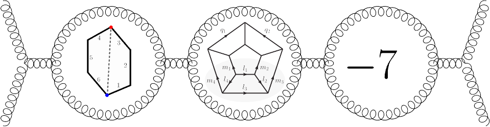
The calculation involved is a little more complicated, but as discovered by Zvi Bern, John Joseph Carrasco, and Henrik Johansson, if you can get your calculation in Yang-Mills into the right format then all you need to do is square the right thing at the right step to get gravity, even for diagrams with loops!

zvi-bern-350

This trick, called BCJ duality after its discoverers, has allowed calculations in quantum gravity that far outpace what would be possible without it. In N=8 supergravity, the gravity analogue of N=4 super Yang-Mills, calculations have progressed up to four loops, and have revealed tantalizing hints that the uncontrolled infinities that usually plague gravity theories are absent in N=8 supergravity, even without adding in string theory. Results like these are why BCJ duality is viewed as one of the “foundational miracles” of the field for those of us who study scattering amplitudes.

Gravity is Yang-Mills squared, in more ways than one. And because gravity is Yang-Mills squared, gravity may just be tame-able after all.

The Parke-Taylor Amplitudes: Why Quantum Field Theory Might Not Be So Hard, After All

2 Replies

If you’ve been following my blog for a while, you know that Quantum Field Theory is hard work. To calculate anything, you have to draw an ever-increasing number of diagrams, translate them into formulas involving the momentum and energy of your particles, and add all those formulas up to get your final result, the amplitude of the process you’re interested in.

As I said in that post, my area of research involves trying to find patterns in the results of these calculations, patterns that make doing the calculation simpler. With that in mind, you might wonder why we expect to find any patterns in the first place. If Quantum Field Theory is so complicated, what insurance do we have that it can be made simpler? Where does the motivation come from?

Our motivation comes from a series of discoveries that show that things really do simplify, often in unexpected ways. I won’t go through all of these discoveries here, but I want to tell you about one of the first discoveries that showed amplitudes researchers that they were on the right track.

Let’s try to calculate a comparatively simple process. Say that we’ve got two gluons (force carrying bosons for the strong force, an example of a Yang-Mills field). Suppose the two gluons collide, and some number of gluons emerge. It could be two again, or it could be three, or more.

For now, let’s just think about diagrams at tree level, that is, diagrams with no loops. The particles can travel from place to place in the diagram, but they can’t form closed loops on the inside.

Gluons have two types of interactions, places where particle lines can come together. You can either have three lines meeting at one point, or four.

If two gluons come in and two come out, we have four possible diagrams:

4ptMHV

Note that while the last diagram looks like it has a loop in it (in the form of the triangle in the middle), actually that triangle just represents that two particles are passing each other without colliding, so that their lines cross.

The number of diagrams increases substantially as you increase the number of outgoing particles. With two particles going to three particles, you get fifteen diagrams. Here are three examples:

5ptMHV

Since the number of diagrams just keeps increasing, you’d expect the final amplitude to become more and more complicated as well. However, Steven Parke and Tomasz Taylor found in 1986 that for a particular arrangement of the spins of the particles (for technical people: this is the Maximally Helicity Violating configuration, or two particles with negative helicity and all the rest with positive helicity) the answer simplifies dramatically. In the sort of variables we use these days, the result can be expressed in an incredibly simple form:

$\frac{\langle 1 | 2 \rangle^4}{ \langle 1 | 2 \rangle\langle 2 | 3 \rangle\langle 3 | 4 \rangle \ldots \langle n-1 | n \rangle\langle n | 1 \rangle}$

Here the angle brackets represent momenta of the incoming (for 1 and 2) and outgoing (all the other numbers) particles, with n being the total number of particles (two going in, and however many going out). (Technically, these are spinor-helicity variables, and those interested in the technical details should check out chapter 3 of this or chapter 2 of this.)

Nowadays, we know why this amplitude looks so simple, in terms of something called B C F W recursion. At the time though, it was quite extraordinary.

This is the sort of simplification we keep running into when studying amplitudes. Almost always, it means that there is some deeper principle that we don’t yet understand, something that would let us do our calculations much faster and more efficiently. It indicates that Quantum Field Theory might not be so hard after all.

Duality: Find out what it means to me

1 Reply

There’s a cute site out there called Why String Theory. Started by Oxford and the Royal Society, Why String Theory contains lots of concise and well-illustrated explanations of string theory, and it even wades into some of the more complex topics like AdS/CFT and string dualities in general. Their explanation of dualities is a nice introduction to why dualities matter in string theory, but I don’t think it does a very good job of explaining what a duality actually is or how one works. As your fearless host, I’m confident that I can do better.

Why String Theory defines dualities as when “different mathematical theories describe the same physics.” How does that work, though? In what sense are the theories different, if they describe the same thing? And if they describe the same thing, why do we need both of them?

You’ve probably seen the above image before, or one much like it. Look at it one way, and you see a goblet. Another, and you see two faces.

Now imagine that instead of a flat image, these are 3D objects, models you have in your house. You’ve got a goblet, and a pair of clay faces. You’re still pretty sure they fit together like they do in the image, though. Maybe they said they fit together on the packaging, maybe you stuck them together and it didn’t look like there were any gaps. Whatever the reason, you’re confident enough about this that you’re willing to assume it’s true.

Now suppose you want to figure out how long the noses on the faces are. In case you’ve never measured a human nose, I can let you know that it’s tricky. You could put a ruler along the nose, but it would be diagonal rather than straight, so you wouldn’t get an accurate measurement. Even putting the ruler beneath the nose doesn’t work for rounded noses like these.

That said, measuring the goblet is easy. You can run measuring tape around the neck of the goblet to find the circumference, and then calculate the diameter. And if you measure the goblet in this way, you also know how long the faces’ noses are.

You could go further, and build up a list of things you can measure on one object that tell you about the other one. The necks match up to the base of the goblet, the foreheads to the mouth, etc. It would be like a dictionary, translating between two languages: the language of measurements of the faces, and the language of measurements of the goblet.

That sort of “dictionary” is the essence of duality. When two theories have a duality (are dual to each other), you can make a “dictionary” to translate measurements in one theory to measurements in the other. That doesn’t mean, however, that the theories are clearly connected: like 3D models of the faces and the goblet, it may be that without looking at the particular “silhouette” defined by duality the two views are radically different. Rather than physical objects, the theories compare mathematical “objects”, so rather than physical obstructions like the solidity of noses we have to deal with mathematical ones, situations where one quantity or another is easier or harder to calculate depending on how the math is set up. For example, many dualities relate things that require calculations at very high loops to things that can be calculated with fewer loops (for an explanation of loops, check out this post).

As Why String Theory points out, one of the most prominent dualities is called AdS/CFT, and it relates N=4 super Yang-Mills (a Conformal Field Theory, or CFT) to string theory in something called Anti-de Sitter (AdS) space (tricky to describe, but essentially a world in which space is warped like a hyperbola). Another duality relates N=4 super Yang-Mills Feynman diagrams with n particles coming in from outside to diagrams with an n-sided shape and particles randomly coming in from the edges of the shape (these latter diagrams are called Wilson loops). In general N=4 super Yang-Mills is involved in many, many dualities, which is a big part of why it’s so dang cool.

Achieving Transcendence: The Physicist Way

5 Replies

I wanted to shed some light on something I’ve been working on recently, but I realized that a little background was needed to explain some of the ideas. As such, this post is going to be a bit more math-y than usual, but I hope it’s educational!

Pi is special. Familiar to all through the area of a circle $\pi r^2$ , pi is particularly interesting in that you cannot write an algebra equation made up of whole numbers whose solution is pi. While you can easily get fractions ( $3x=4$ gives $x=\frac{4}{3}$ ) and even many irrational numbers ( $x^2=2$ gives $x=\sqrt{2}$ ), pi is one of a set of numbers that it is impossible to get. These special numbers transcend other numbers, in that you cannot use more everyday numbers to get to them, and as such mathematicians call them transcendental numbers.

In addition to transcendental numbers, you can have transcendental functions. Transcendental functions are functions that can take in a normal number and produce a transcendental number. For example, you may be aware of the delightful equation below:

$e^{i \pi}=-1$

We can manipulate both sides of this equation by taking the natural logarithm, $\ln$ , to find

$i\pi=\ln(-1)$

This tells us that the natural logarithm function can take a (negative) whole number (-1) and give us a transcendental number (pi). This means that the natural logarithm is a transcendental function.

There are many other transcendental functions. In addition to logarithms, there are a whole host of related functions called the polylogarithms, and even more generally the harmonic polylogarithms. All of these functions can take in whole numbers like -1 or 1 and give transcendental numbers.

Here physicists introduce a concept called degree of transcendentality, or transcendental weight, which we use to measure how transcendental a number or a function is. Pi (and functions that can give pi, like the natural logarithm) have transcendental weight one. Pi squared has transcendental weight two. Pi cubed (and another number called $\zeta(3)$ ) have transcendental weight three. And so on.

Note here that, according to mathematicians, there is no rigorous way that a number can be “more transcendental” than another number. In the case of some of these numbers, like $\zeta(5)$ , it hasn’t even been proven that the number is actually transcendental at all! However, physicists still use the concept of transcendental weight because it allows us to classify and manipulate a common and useful set of functions. This is an example of the differences in methods and standards between physicists and mathematicians, even when they are working on similar things.

In what way are these functions common and useful? Well it turns out that in N=4 super Yang-Mills many calculated results are not only made up of these polylogarithms, they have a particular (fixed) transcendental weight. In situations when we expect this to be true, we can use our knowledge to guess most, or even all, of the result without doing direct calculations. That’s immensely useful, and it’s a big part of what I’ve been doing recently.

Ansatz: Progress by Guesswork

4 gravitons

Stories about physics from someone who's been there